Adams Car Dynamic Suspension Analysis
This example demonstrates the ability to carry out Dynamic Suspension Analysis. Instead of using a quasi-static simulation the suspension assembly is simulated with the Adams Solver Simulate/Dynamic command.
This feature allows you to directly provide a RPCIII file or define View Functions to specify Jack and Steering motion as a function of displacement, force and so on.
Model Description
A Suspension Assembly consisting of a double wishbone suspension and a rack and pinion steering system is provided. A dynamic suspension analysis is carried out to actuate the wheel pads across a range of frequencies. We are interested in looking at the lower control arm bushing force and how the force changes by replacing the rigid lower control arm by a flexible body. In addition, we use the flex body swap dialog box to switch a rigid lower control arm with a flexible one. We then plot the stress on the flexible body node and visualize it. |  |
Investigate the model and carry out a Dynamic Analysis
Here you first analyze a double wishbone suspension with rigid lower control arm
1. Start Adams Car, select Standard Interface.
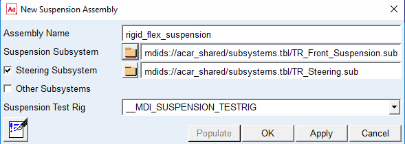
2. Create a new Suspension assembly: File → New → Suspension Assembly. Fill the dialog box as indicated below. To select the subsystems, Right click → Search → <acar_shared> to open the file browser.
3. The suspension assembly should be displayed.
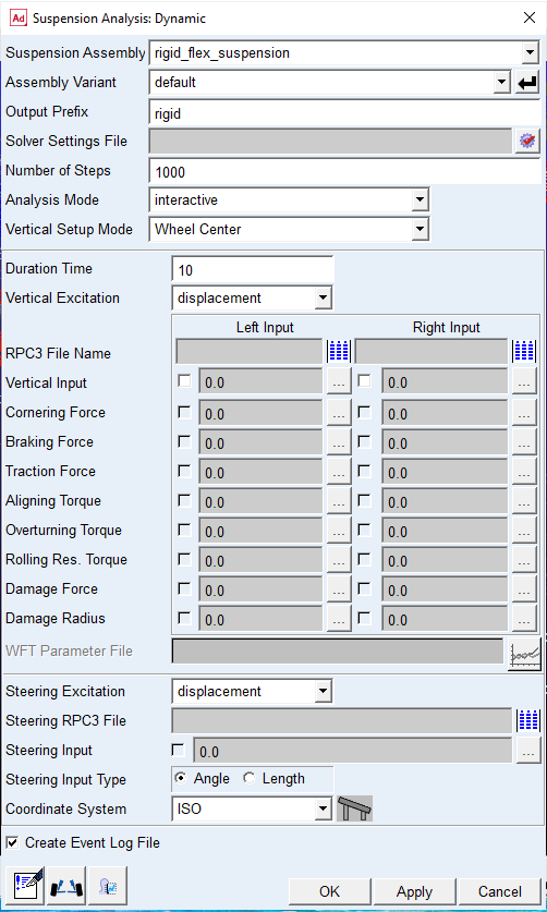
4. To simulate using the Dynamic Solver Statements, go to Simulate → Suspension Analysis → Dynamic.
5. To animate the results, from the Review menu, select Animation Controls. Animate the model and observe the change in the suspension travel.
Review the results
Plot the bushing force in the lca_front bushing:
1. Press the F8 key in Adams Car to switch to Adams PostProcessor.
2. Locate the bkl_lca_front_force and bkr_lca_front_force REQUEST under user-defined REQUESTs:
The fz_front component corresponds to magnitude of the force in the Z direction. Plot this quantity to obtain a figure similar to the following:
Change Rigid Lower Control arm to be a Flexible Body
Here you use the Flex body Swap dialog box feature available in the Standard interface to replace the left rigid lower control arm with a flexible body. The MNF file used for representing this flex body is created in Nastran.
To replace the lower control arm:
1. Go to Adjust → General Part → Rigid to Flex. This displays the flex body swap dialog box.
2. Right click the Current Part Field - Pick and select the Left Lower control arm. In the MNF File field, Right-click → Search → <acar_shared>\flexbodys.tbl and select the LCA_left_tet.mnf file.
3. Click on the Connections tab and highlight the Align column and select Preserve Marker Expression and click OK.
4. Now, the rigid lower control arm in red is replaced by the white flexible body.
Simulate the Model
You again carry out a dynamic analysis with this model now containing a flexible body.
1. Go to Simulate → Suspension Analysis → Dynamic.
2. Name the Output Prefix to be Rigid_Flex and keep the remaining dialog box unchanged.
After the simulation is successful, animate the model to make sure it is behaving as expected.
Review & Compare Results
Here you plot the bushing force for the lower control arm and compare the force on left and right side.
To review the results:
1. Locate the bkl_lca_front_force and bkr_lca_front_force REQUEST under user-defined REQUESTs:
2. Because of the left lower control arm being a flexible body, note the difference in the bushing force.
Optional: Load Durability Plugin to display Stresses and Identify the Hotspots
Here you will load the Durability Plugin and identify the hot-spots on the flexible lower control arm and also plot the nodal stresses. For better visualization, in the Adams Car Standard Interface change the background color from Black to Gray (Settings - View Background Color).
To Display Stresses and animate the flex body:
1. Change to Adams Postprocessor and switch to Animation mode.
2. Go to View → Load Animation and select Rigid_Flex_dynamic to load the animation.
3. Go to Tools → Plugin Manager and check the load Adams Durability option.
4. In the Animation tab right click the Component field and select the flexible body gel_lower_control_arm_flex. This only displays the flexible body and not the whole model.
5. Select the Contour Plots tab; set Contour Plot Type to Von Mises Stress and check Display Legend.
6. Select the Hot Spots tab; check Display HotSpots and fill the dialog box as shown below. You are interested in looking at the top 2 hotspots on the flexible body.
7. Play the animation; you would observe the change in stress with the hot spots being identified.
8. From the above exercise, you can note that Node with ID 709 experiences the maximum Von Mises Stress. You can now, plot the stress at this node. Go to Durability menu at the top and select Nodal Plots. The dialog for Nodal Plots pops up. In the Select Node List field, fill in 709, Check Von Mises and click OK.
9. Switch back to Plotting mode in the Adams PostProcessor, Set the Source to be Result Sets; select gel_lower_control_arm_flex_Stress and component to be node_709_Von_Mises. Your plot should look something like shown below.
Remarks
■The above example, demonstrates a simple use of applying a non standard excitation to a suspension assembly. You could use an RPCIII file from test data to actuate your suspension or use other Adams View functions. An example RPCIII file (roadprofile_lr_channels.drv) has been provided in the shared car database with your Adams installation (install_dir\acar\shared_car_database.cdb\loadcases.tbl).
■While animating or during plotting of the hot spots/stresses for the first time, you may see a progress bar. This is showing the caching of the Flex Cache Files for improving performance for future animation and post processing.