Important Simulation Settings
There are a few settings to be aware of when simulating Adams models which include nonlinear flexible bodies:
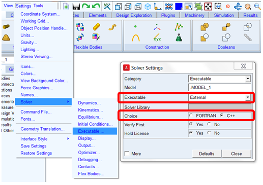
■Executable: Adams models containing nonlinear flexible bodies cannot be solved via the Adams View internal solver, which is the default. Only external Adams Solver launched from Adams View or standalone Adams Solver can be used. This can be set within Adams View from the Settings menu - Solver - Executable dialog's "Executable" option menu. Select "External" or "Files Only." Note that in Adams Car, "External" is the default. Also note that Adams models containing nonlinear flexible bodies can only be solved by Adams Solver (C++), which is the default for internal and external simulations launched from Adams View and Adams Car.
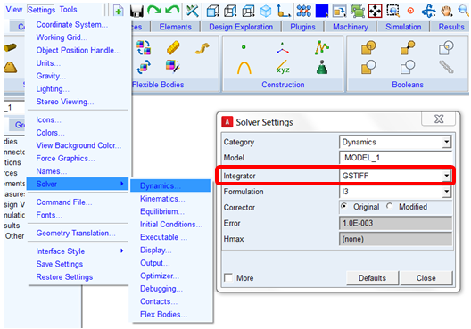
■Integrator: Currently models containing nonlinear flexible bodies submitted for dynamic analysis can only be solved via the GSTIFF or HHT integrators. GSTIFF is the default setting. The setting can be verified within Adams View from the Settings menu - Solver - Dynamics:
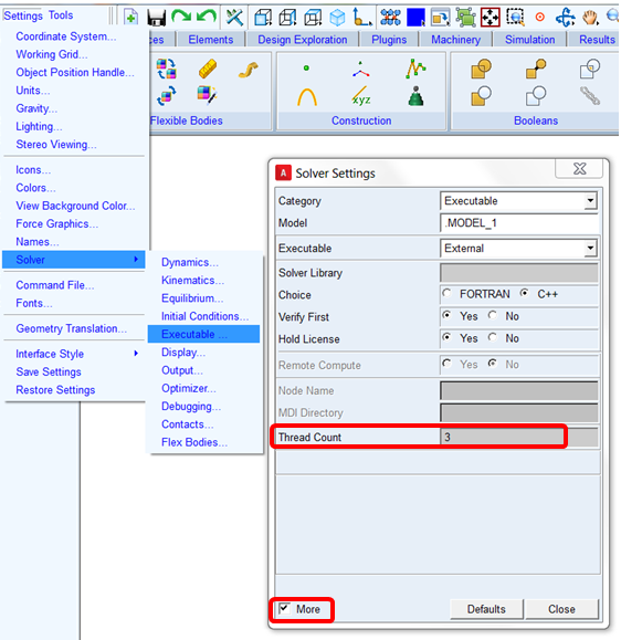
■Adams Solver Thread Count: In general this setting can be very beneficial to solve times when simulating large Adams models on machines with multiple CPU's. This is also true for models with multiple nonlinear flexible bodies. Often the nonlinear flexible bodies will be, by far, the most computationally intensive portions of the overall Adams model. By increasing the Adams Solver thread count, Adams Solver will place each nonlinear flexible body on separate threads so they can be solved in parallel. This can be set within Adams View from the Settings menu - Solver - Executable - More:
When the model has only one nonlinear flexible body there might not much benefit to this unless the rest of the Adams model is not insignificant in complexity by comparison (otherwise large number of degrees of freedom, number of parts, contacts and so on.). This is because the rest of the Adams model will solve so quickly compared to the single nonlinear flexible body that there will be little benefit of separating the two portions of the analysis. To reduce solution time for any one nonlinear flexible body in the model use the nonlinear flexible body number of threads instead which can be effective for relatively large nonlinear flexible bodies (~500,000 nodes or more). See "Guidelines on Thread Count Usage" below for more details.
■Guidelines on Thread Count Usage: The Adams Solver thread count is separate and distinct from the Number of Threads which can be assigned per nonlinear flexible body via the nonlinear flexible body modify dialog here:
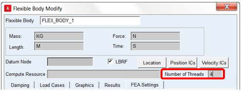
While the Adams Solver thread count will ensure that each of the nonlinear flexible bodies in the model are solved in parallel to each other (and possibly the rest of the Adams model), the nonlinear flexible body's "Number of Threads" setting will break down the solving of each flexible body so that it can be parallelized itself and further performance improvements are possible. Currently no more than 4 threads per nonlinear flexible body is recommended since beyond that the performance of the flexible body typically stops improving and, in fact, can degrade. Furthermore, increasing the nonlinear flexible body's "Number of Threads" will only show significant performance improvement if the nonlinear flexible body is relatively large (~500,000 nodes or more). See the table below for suggested thread count settings for some example model configurations:
Size/complexity of Adams model aside from NL flex bods | Number of relatively large NL flex bods | Number of relatively small NL flex bods | Suggested Adams Solver Thread Count | Suggested Number of Threads (large NL flex bods) | Suggested Number of Threads (small NL flex bods) |
|---|---|---|---|---|---|
small | 1 | 0 | 1 | 4 | - |
large | 1 | 0 | 2 | 4 | - |
small | 1 | 2 | 3 | 4 | 1 |
large | 1 | 2 | 4 | 4 | 1 |
small | 0 | 3 | 3 | - | 2-4 |
Note: | These are general examples intended only to help illustrate the distinction between Adams Solver Thread Count and the Nonlinear Flexible Body's Number of Threads and how they might be used to improve performance. The optimal settings in reality will depend on the specify model and the number of CPU's on the machine(s) running the simulations. |
■Integration Error Tolerance: The Adams user is able to specify the local integration error tolerances that the integrator must satisfy at each step independently for the Adams multibody system and the nonlinear flexible body. Typically, in the case of the Adams multibody system, only one local integration error tolerance can be specified for the whole set of differential and algebraic equations (DAE), which are integrated at each time step. For more details see the description of "Error" in the INTEGRATOR statement documentation in the Adams Solver C++ Help.
In case of models containing a nonlinear flexible body, the MSC Nastran-type error tolerance for its states can be set independently. By default the nonlinear flexible body sets the following parameters in the run-ready MSC Nastran data deck (.dat) written out by Adams View or Adams Car:
PARAM, CSERRTYP, 0
PARAM, CSOERR, 1.0E-3
This setting specifies an error tolerance of 0.001 which is used in the corrector convergence criteria of MSC Nastran O-set states. Note that looser tolerance can speed up the simulation but may lead to less accurate results. On the other hand, tighter tolerance can provide better results but may lead to higher number of Newton-Raphson iterations and a possible incapability to meet the required corrector convergence criteria (that is, corrector failure). The default value is 1.0E-3.
As a second option, the user can set an Adams-type error criteria by setting the following parameters:
PARAM, CSERRTYP, 1
PARAM, CSERRSCA, 1.0E3
This setting specifies a scale factor of 1.0E3 for the Adams corrector convergence tolerance. The 'scaled' tolerance is used in the corrector convergence criteria of MSC Nastran O-set states. In this setting Adams-type corrector convergence criteria is used for all the states in a model. Note that the original corrector convergence tolerance is used for Adams states and the scaled tolerance is used for the nonlinear flexible body states. A good rule of thumb is to use a scale factor of 1.0E3.
■PATTERN for Jacobian Reevaluation: In case of a model with a nonlinear flexible body, the following default pattern is used for reevaluating the Jacobian matrix for Newton-Raphson iteration in GSTIFF and HHT integrators:
INTEGRATOR/PATTERN = T:F:F:F:T:F:F:F:T:F
The ratio 1/4 (1 reevaluation each 4 nonlinear iterations) is the most adequate for normal simulation, with a good compromise between performance and ability to converge in Newton-Raphson.
However, in the case of following conditions:
♦Large plastic deformation
♦Self-contact in the nonlinear flexible body
♦Hyperelastic material
…it is advised to force the reevaluation at each nonlinear iteration, with the following command:
INTEGRATOR/PATTERN = T
This setting forces the Jacobian matrix to be reevaluated at each Newton-Raphson iteration. The simulation time may be penalized, but it is required to achieve corrector convergence in the above conditions.
■Guidelines when Using Self Contact in Nonlinear Flexible Body: In case of a model having a nonlinear flexible body undergoing self-contact we recommend:
a. Forced Jacobian reevaluation at each nonlinear iteration with the following command:
INTEGRATOR/PATTERN = T
This is due to the fact that boundary condition in a self-contacting NLFE body change abruptly during self-contact.
b. As contact is an inherently non-linear and non-smooth phenomena it may be necessary to limit the maximum step size taken by the integrator. This may be done by using the hmax option in the integrator command:
INTEGRATOR/HMAX=1.0E-04
c. To request the contact output and monitor its status, by default, we add the BOUTPUT case control statement to the run-ready MSC Nastran data deck (.dat) written out by Adams View or Adams Car for each nonlinear flexible body specified to use self-contact as follows:
BOUTPUT(PRINT,PLOT) = ALL
If this statement is present in the run-ready MSC Nastran data deck (.dat), then the Adams console and .msg file will output information messages when self-contact begins and ends. Additionally, the output histories (contact forces and stresses) of contact nodes are output in text form to the .f06 file and in plot form (which can viewed in an FE postprocessor) to the op2 file.
■Simulation Time Reported: The elapsed time and CPU time reported at the end of the Adams Solver message file (.msg) reflects the time the entire analysis took. To determine the portion of that time consumed only by any one nonlinear flexible body in the Adams model, one can open the .sts file corresponding to that nonlinear flexible body and look near the bottom of the file. The file can be found in the working directory and its name is a combination of the Adams analysis files' name and the nonlinear flexible body's name.