Create Precompute TestRig
Machinery -> Gear -> Create Precompute TestRig 
For the option | Do the following |
|---|---|
Module (Normal Plane) | Enter a value for the module expressed in the normal plane (MN). The module is the pitch diameter divided by the number of teeth. |
Pressure Angle (Normal Plane) | Enter a nominal pressure angle (α) in current modelling Units (default value = 20.0 deg) expressed in the normal plane. The angle between the line of action and the common tangent to the pitch circles at the pitch point is the pressure angle. 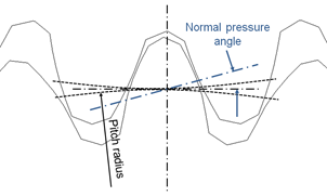 |
Helix Angle | The helix angle defines the slope of the tooth in lead direction against the rotational axis at the pitch diameter. A positive sign corresponds with the right hand rule. A straight spur gear has a helix angle of zero. 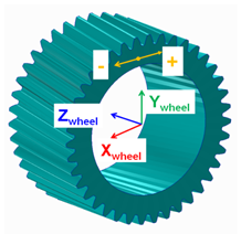 |
File Name | Enter the file name. |
GEAR PAIR | |
FGF Input | Gear profile data can be migrated using .FGF. |
General | |
Number of Teeth | Number of Teeth on Gear 1 and 2. Negative number in FGF or DAT indicates internal gear. |
Addendum Mod.Coefficient (X) | This factor is positive, when the reference profile is moved into the direction of the tip of the tooth by the product module * factor. |
Rim/Bore Diameter | The rim diameter for an external gear and the bore diameter for an internal gear define the boundary of the gear rim. Meshing is done upto rim/bore diameter to generate .SHL file. If bore or rim diameter are specified as zero, then those are auto calculated as: Bore / rim diam = root circle diam -/+ 0.5 * module 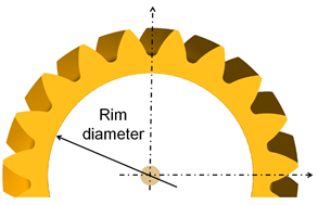 |
Gear Width | Each gear wheel has a reference marker in the middle of the gear rim with width 'w'. The z-axis of this reference marker represents the rotation axis of the gear wheel. 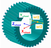 |
Tooth Profile | |
Tooth Flank | |
Tip Chamfer Length Factor | The angle of the chamfer is calculated in such a way, that the inclination between involute and chamfer and between tip radius and chamfer is equal. The intersection of the chamfer with the involute defines 'end contact'. 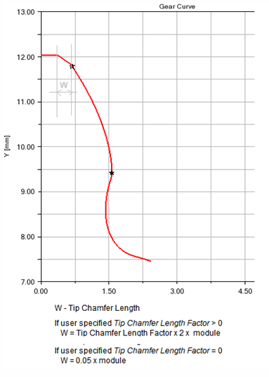 |
Tip Fillet Radius | If the input is greater than zero, a radius is created and an eventually Tip Chamfer defined above is ignored. The fillet is tangent with the 'end contact'. |
Root Fillet Radius Factor | This factor multiplied by the normal module delivers the fillet radius at tooth root. The intersection with the involute defines Start Contact. |
Addendum Mod. Factor | The tooth tip height results from the multiplication of the 'normal module' by this factor. The height is measured from the pitch circle. |
Dedendum Mod. Factor | The tooth root height results from the multiplication of the 'normal module' by this factor. The height is measured from the pitch circle. |
Cutter Rack | |
Tip Clearance Factor | The factor multiplied by normal module delivers the additional clearance, which is an outcome of the increased rack tip height |
Protuberance Radius | The radius at the tip of the protuberance tool. 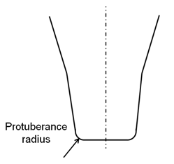 |
Protuberance Length | Length measured from Rack Tip as shown: 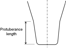 |
Protuberance Angle | The angle of the protuberance is measured against the symmetry plane of the tooth on the rack. 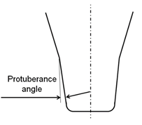 |
Protuberance Thickness | This thickness can be used to simulate the grinding tool, which is removing material from the tooth flanks produced by the rack. 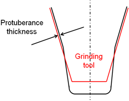 |
Involute | |
Barreling Coefficient | The involute modifications support barreling applied to left/right flank as shown below: 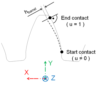 Barreling (hbarrel) is defined as a cubic function of the dimensionless variable u (in radial direction) through equations: u = ( radius - radiusstart ) / (radiusend - radiusstart) hbarrel = a1 * u + a2 * u**2 + a3 * u**3 |
Involute Slope | The involute slope is also applied to the left and to the right flank. The slope is defined through the angle  involute. The angle is positive in material-in wise direction as shown below (right flank): involute. The angle is positive in material-in wise direction as shown below (right flank):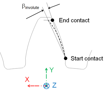 |
Tooth Modification | |
Tip and Root Modification | |
Tip Relief Coeff. | Tip Relief Length and Root Relief Length define the diameter, where the relief starts. Tip and Root relief modifications can be applied for the left and/or the right flank. Both reliefs are defined by a cubic polynomial htip = a1 * utip + a2 * utip**2 + a3 * utip**3 hroot = b1 * uroot + b2 * uroot**2 + b3 * uroot**3 where, dimensionless variables utip and uroot are: utip = (diameter - tip_relief_length ) / ( diameter_end_contact - tip_relief_length ) uroot= (root_relief_length - diameter) / ( root_relief_length - diameter_start_contact) 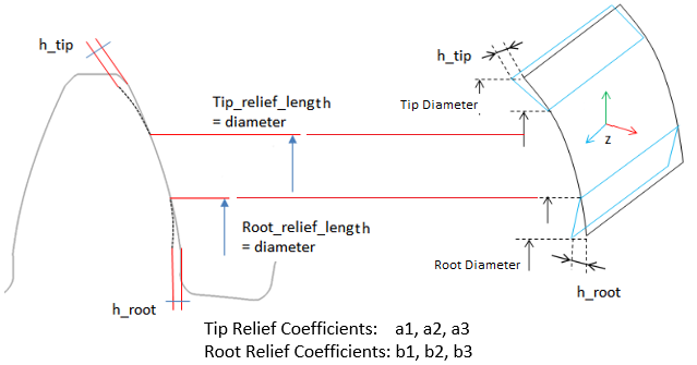 |
Tip Relief Lengh | |
Root Relief Coeff. | |
Root Relief Length | |
Lead Modification | |
Crowning Coefficients | Crowning is applied in a plane xp-zp, which is perpendicular to the contour of the tooth. Crowning hcrown is defined as a cubic function of a dimensionless variable u. 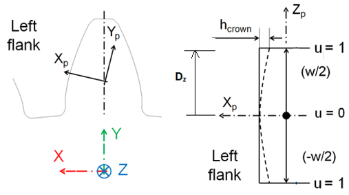 The dimensionless variable u follows from equation: u = |zp| / (w/2) The cubic polynomial is given in equation hcrown = a1 * u + a2 * u**2 + a3 * u**3 Following equation gives the relation between the crowning drop hcrown and crowning radius R. R = ( (w/2) **2 + hcrown**2 ) / ( 2 * hcrown) Generally hcrown is very small compared to the width of the rim; so equation below should be a valid approximation for a circular crowning: a2 = hcrown; a1 = a3 = 0.0 Crowning h1 at u=u1 ( u1 > 0.0 and u1 < 0.0) and h2 at u=1.0 with no slope at u=0 is defined by the coefficients of equations: a1 = 0 a2 = ( h1 - h2 * u1**3 ) / ( u1**2 - u1**3 ) a3 = ( h2 * u1**2 - h1 ) / ( u1**2 - u1**3 ) |
End Relief +ve Length End Relief +ve Coeff. End Relief -ve Length End Relief -ve Coeff. | The relief lengths lpos and lneg define the width, where the modification is applied. A dimensionless variable u is introduced to facilitate input for the end relief modifications: 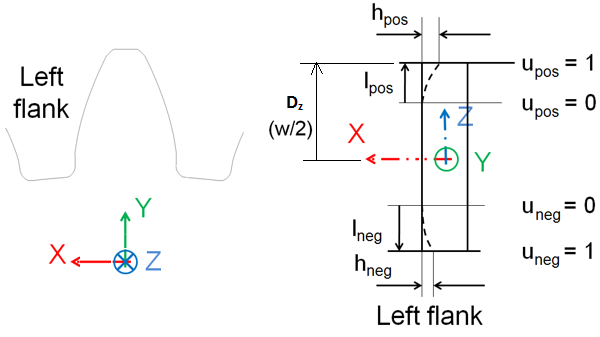 Following equations show the dimensionless variable u. upos = ( zrim - ( gear_width/2 - lpos ) ) / lpos uneg = ( |zrim| - ( gear_width/2 - lneg ) ) / lneg In correlation with crowning, a cubic polynomial from equations below defines the relief. hpos = b1 * u + b2 * u**2 + b3 * u**3 hneg = b1 * u + b2 * u**2 + b3 * u**3 Equations below give the relation between the end reliefs hpos and hneg and a corresponding radius. Rpos = ( (lpos**2 + hcrown**2 ) / ( 2 * lpos ) Rneg = ( (lneg**2 + hcrown**2 ) / ( 2 * lneg ) Generally the relief is small compared to the length of the relief, what allows to approximate the radius by equations b2pos = lpos ; b1 = b3 = 0.0 b2neg = lneg ; b1 = b3 = 0.0 Relief h1 at u=u1 ( u1 > 0.0 and u1 < 0.0) and h2 at u=1.0 with no slope at u=0 is defined by the coefficients of equations: b1 = 0 b2 = ( h1 - h2 * u1**3 ) / ( u1**2 - u1**3 ) b3 = ( h2 * u1**2 - h1 ) / ( u1**2 - u1**3 ) |
Lead Slope | The lead slope  (in degrees) defines a correction with respect to the helix angle as seen in figure below: (in degrees) defines a correction with respect to the helix angle as seen in figure below: 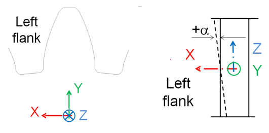 The principles for lead modifications are identical between left and right flank. The only point of attention is the definition of the lead slope as shown as: 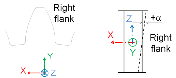 |
Mass | |
Mass | Enter the mass of the gear part. |
The parts are located at the center of the gear, with the z-axis as the rotational axis. | |
Inertia | |
Ixx/Iyy/Izz | Enter the values that define the principal mass-inertia components of the gear part. |
Ixy/Izx/Iyz | Enter the values that define the deviational (cross-product) mass-inertia components of the gear part. |
CM Location Relative to Part | Enter the value relative to the part. |
Young’s Modulus | Young's modulus E defines the relation between tensile strain  and tensile stress and tensile stress  by Hooke's law: by Hooke's law:  |
Poisson’s Ratio | An extension  of a linear elastic and isotropic material is accompanied by lateral strains of a linear elastic and isotropic material is accompanied by lateral strains  and and  . Poisson's ratio . Poisson's ratio  defines this relation by equations: defines this relation by equations:  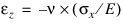 Or 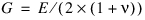 where G is shear modulus. where G is shear modulus. |
Material Density | The mass m of a solid body is computed by equation its volume V multiplied by the mass density  . .  |
Mesh Properties | |
Mesh Density | Mesh density defines the number of finite elements along the contact line. 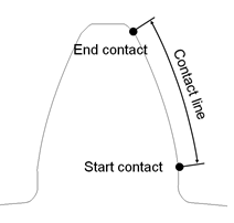 The contact line represents the portion of the profile (flank), where contact is supported. The contact line is defined through start contact and end contact: Start contact is close to the root for external and internal gears. Valid input entries for mesh density are 1 to 5, meaning 16,24,32,40 or 48 elements along the contact line. This input parameter allows you to select your preference with respect of accuracy versus CPU-time. A low value for mesh density will result in a coarser Nastran model, what gives generally a short CPU-time. One has to keep in mind, that a coarse model is generally slightly stiffer. The accuracy of the contact computations in Adams by the Gear AT force is not influenced strongly in quality and in CPU-time by mesh density, as the contact algorithm uses an accurate definition of the tooth flank surface. It is recommended that both meshing gears should have same mesh density. |
No. of Contact Planes | The integer value of number of contact planes divides the width of a tooth into a number of equidistant sections in lead direction. It is suggested, number of contact planes should be same on both gears in mesh. Contact between gear wheels is checked at each 'contact plane' of wheel 1 of the Gear AT force. A too small number of contact planes may be leading to some numerical noise. CPU time increases with increasing number of contact planes. You need to verify the appropriateness of your selection. Following default values are implemented: u = width / ( 2 * module * 10 ) number contact planes = 20 * ( 1 - u ) + 30 * u |
Load Element Size | Load Element Size defines the number of finite elements in lead direction per section. The length of the section is given by 'width' divided by 'number of contact planes'.  A larger number of this input will increase the size of the FE-mesh and hence the CPU-time of the Nastran analysis. |
Display Ratio Lead | The SHELLs are used for the display only; they are not used for any contact simulation. The input for Display Ratio Lead defines number of divisions for Shell geometry in lead direction as a fraction of contact planes number. Value 2 means half the number of divisions to the number of contact planes. 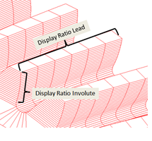 |
Display Ratio Involute | The SHELLs are used for the display only; they are not used for any contact simulation. The input for display ratio involute defines number of divisions for shell geometry in involute direction as a fraction of contact elements number defined by mesh density. Value 2 means half the number of divisions to the number of contact elements. |
GCP Creation The below options helps you to create GCP file which contains all necessary data for precomputed contact. The data is generated automatically by a test rig. The preprocessing starts with automated building of gear pair test rig in the background. You need to provide an input for both the gears (or refer to an existing FGF to fill up GUI). 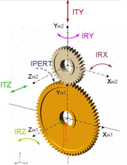 The test rig create FGP files for both the gears and uses those files for simulation with the specified excitation (radial, axial and so on.) | |
Workspace To support misalignments, you need to fill the entries in group Workspace. Misalignments are applied symmetrically, relatively to the initial position of the secondary wheel, the smaller gear in picture. | |
Radial Displacement | Radial Displ., Dist. 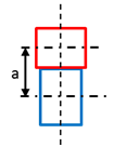 Enter explicitly axial distance between the gear wheels. In case the testrig is extracted from existing model the axial distance is taken from the model, for case the model is assembled manually the axial distance is suggested. For zero value the entry is ignored. Radial Displ. 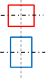 Defines range for radial distance variations from initial position. The range is defined symmetrically to the initial position by value 'Perturbation' and for 'Steps' *2 + 1 discrete positions resp. -'Steps' to + 'Steps' including zero deviation. Corresponds to ITY on Figure. |
Axial Displacement | Axial Displ. 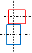 Defines range for translations in direction of rotational axis from initial position. It is assumed the initial offset between gear centers is zero. Corresponds to ITZ on Figure. |
Lateral Misalignment | Lateral Misalignment 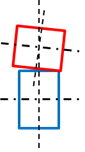 Defines range for inclination angles about x axis of contact coordinate system from initial position. Corresponds to IRX on Figure. |
Radial Misalignment | Radial Misalignment 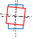 Defines range for inclination angles about y axis of contact coordinate system from initial position. Corresponds to IRY on Figure. Radial Displacement corresponds to ITY translational direction and is applied relative to actual axial distance of gears; this distance can be corrected or set in the input box left to the step entry, if zero is specified, the default axial distance is used. Axial Distance corresponds to ITZ translational direction, Lateral Misalignment corresponds to IRX rotation and Radial Misalignment corresponds to IRY rotation of secondary gear wheel. The entries in Step field effectively define Step * 2 + 1 total steps starting from - Perturbation and going to + Perturbation for every workspace dimension. |
Calculation Options | |
Number of steps/halp_pitch | Defines the discretization along the pitch angle of the primary wheel 1. During the preprocessing the gears are rotated from -wheel 1 pitch angle half to + wheel 1 pitch angle half to capture the contact at different relative positions of gear wheels. The total number of positions is equal to 'Number of steps' * 2 + 1. |
Torque | Defines maximum applied torque at every workspace position. The torque is applied in number of steps defined in entry Steps/Workspace dimensions and corresponds to IPERT rotation. If the launched preprocessor produces *.gcp file with no misalignment effects then, this can be used for simple concept studies with rigid shafts and kinematic joints. |
Steps/Workspace dimensions | Enter the number of steps. |
Mirror Minus Mode | The toggle Mirror Minus Mode allow you to skip free play calculations for right / minus flank and just mirror the results of left / plus flank calculations. |
Simulate Test Rig  | Run button automatically launch preprocessor. Calculated data are progressively stored to *.GCP file. The preprocessor starts the calculations with so called "Free play study". In this study the algorithm finds the difference between ideal kinematic and start of the contact position for every defined workspace dimension combination. Teeth profiles symmetrical along vertical axis of tooth cross section have symmetrical free play results for left and right tooth flank, what enables to save computational time in free play study. The simulation progress can be followed in content of *.log file, which shares the same name as the *.gcp file. The log file starts with estimate of required iteration number to be performed and adequate time estimate for the preprocessing. Next sections of log file content informs about progress of free play study, results of the free play study and also about current iteration step and details about contact computation at given workspace position. After the preprocessing is accomplished, the complete GCP file is prepared to be used in simulation. The GCP file has ASCII text format, you can preview them using text editor. |