Modify Advanced 3D Gear Element
For the option | Do the following |
|---|---|
Gear Element Name | Selected gear element name displayed. |
Axis of Rotation | Axis of Rotation of Gear 1 and Gear 2 can be one of the following: ■Orientation ■Pick (Marker) ■Global Z ■Global X ■Global Y |
Center Location | Enter the coordinates or Pick (Markers, View location and so on.) |
FGF Input | Gear profile data can be migrated using .FGF. |
General | |
Number of Teeth | Number of Teeth on Gear 1 and 2. Negative number in FGF or DAT indicates internal gear. |
Addendum Mod.Coefficient (X) | This factor is positive, when the reference profile is moved into the direction of the tip of the tooth by the product module * factor. |
Pressure Angle (Normal Plane) | Enter a nominal pressure angle (α) in current modelling Units (default value = 20.0 deg) expressed in the normal plane. The angle between the line of action and the common tangent to the pitch circles at the pitch point is the pressure angle. |
Helix Angle | The helix angle defines the slope of the tooth in lead direction against the rotational axis at the pitch diameter. A positive sign corresponds with the right hand rule. A straight spur gear has a helix angle of zero. 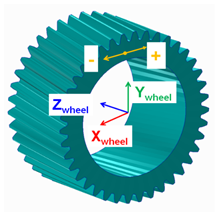 |
Tip Diameter | Enter a value for the tip diameter. |
Root Diameter | Enter a value for the root diameter. |
Rim/Bore Diameter | The rim diameter for an external gear and the bore diameter for an internal gear define the boundary of the gear rim. Meshing is done upto rim/bore diameter to generate .SHL file. If bore or rim diameter are specified as zero, then those are auto calculated as: Bore / rim diam = root circle diam -/+ 0.5 * module 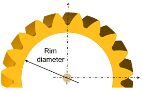 |
Gear Width | Each gear wheel has a reference marker in the middle of the gear rim with width 'w'. The z-axis of this reference marker represents the rotation axis of the gear wheel. 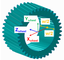 |
Module | Enter a value for the module. |
No. of Teeth to Export | Number of teeth for visualization (SHL geometry). The entry influence also update of inertia tensor of the gear wheel. Hence, it is advised to use 'user specified' mass properties when the number of teeth exported are different than actual. |
Gear Type | ■Internal ■External |
Geometry File | User specified geometry file import for visualization. Mesher generates a .shl file for gear. |
Tooth Profile | |
Tooth Flank | |
Tip Chamfer Length Factor | The angle of the chamfer is calculated in such a way, that the inclination between involute and chamfer and between tip radius and chamfer is equal. The intersection of the chamfer with the involute defines 'end contact'. 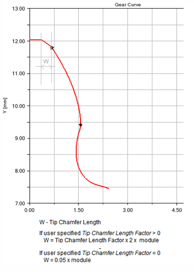 |
Tip Fillet Radius | If the input is greater than zero, a radius is created and an eventually Tip Chamfer defined above is ignored. The fillet is tangent with the 'end contact'. |
Root Fillet Radius Factor | This factor multiplied by the normal module delivers the fillet radius at tooth root. The intersection with the involute defines Start Contact. |
Addendum Mod. Factor | The tooth tip height results from the multiplication of the 'normal module' by this factor. The height is measured from the pitch circle. |
Dedendum Mod. Factor | The tooth root height results from the multiplication of the 'normal module' by this factor. The height is measured from the pitch circle. |
Cutter Rack | |
Tip Clearance Factor | The factor multiplied by normal module delivers the additional clearance, which is an outcome of the increased rack tip height |
Protuberance Radius | The radius at the tip of the protuberance tool. 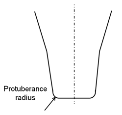 |
Protuberance Length | Length measured from Rack Tip as shown: 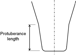 |
Protuberance Angle | The angle of the protuberance is measured against the symmetry plane of the tooth on the rack. 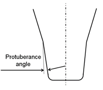 |
Protuberance Thickness | This thickness can be used to simulate the grinding tool, which is removing material from the tooth flanks produced by the rack. 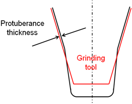 |
Involute | |
Barreling Coefficient | The involute modifications support barreling applied to left/right flank as shown below: 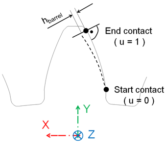 Barreling (hbarrel) is defined as a cubic function of the dimensionless variable u (in radial direction) through equations: u = ( radius - radiusstart ) / (radiusend - radiusstart) hbarrel = a1 * u + a2 * u**2 + a3 * u**3 where, a1, a2 and a3 are barreling coefficients |
Involute Slope | 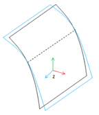 Involute slope is used to compensate for tooth deflection differences between the two meshing gears and to compensate for system deflections that would otherwise result in hard contact near the root or the tip of one of the gears. The involute slope is also applied to the left and to the right flank. The slope is defined through the angle  involute. The angle is positive in material-in wise direction as shown below (right flank): involute. The angle is positive in material-in wise direction as shown below (right flank):  |
Tooth Modification | |
Tip and Root Modification | |
Tip Relief Coeff. | tip telief length and root relief length define the diameter, where the relief starts. Tip and root relief modifications can be applied for the left and/or the right flank. Both reliefs are defined by a cubic polynomial htip = a1 * utip + a2 * utip**2 + a3 * utip**3 hroot = b1 * uroot + b2 * uroot**2 + b3 * uroot**3 where, dimensionless variables utip and uroot are: utip = (diameter - tip_relief_length ) / ( diameter_end_contact - tip_relief_length ) uroot= (root_relief_length - diameter) / ( root_relief_length - diameter_start_contact) 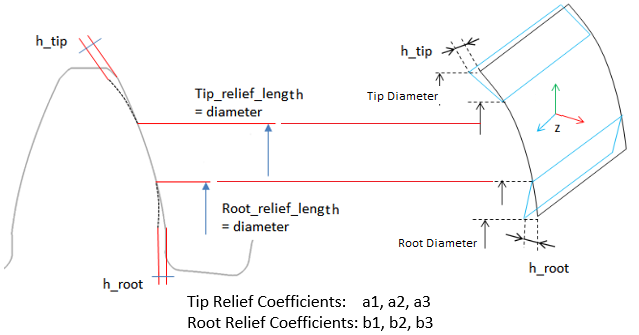 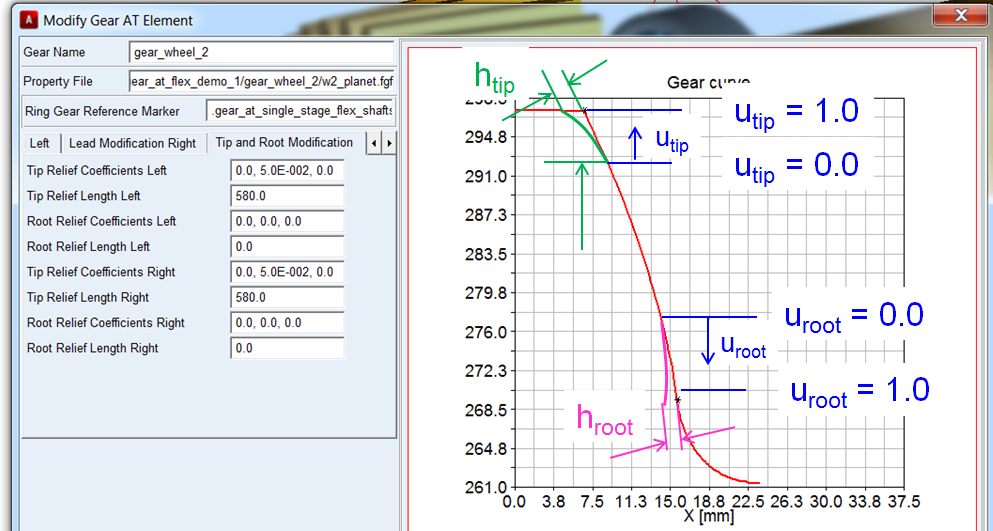 |
Tip Relief Lengh | |
Root Relief Coeff. | |
Root Relief Length | |
Lead Modification | |
Crowning Coefficients | 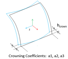 Crowning is convex shape along the width of a tooth. It is used to maintain contact in the central region of the tooth flank width allowing for gear angular and axial misalignment. This type of tooth modification is preferably used on narrow gears. The amount of crowning should not be larger than necessary as otherwise it would reduce area of contact, thus lowering load capacity of a gear pair. Crowning is applied in a plane xp-zp, which is perpendicular to the contour of the tooth. Crowning hcrown is defined as a cubic function of a dimensionless variable u. 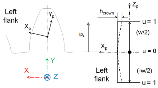 |
The dimensionless variable u follows from equation: u = |Dz| / (w/2) The cubic polynomial is given in equation hcrown = a1 * u + a2 * u**2 + a3 * u**3 Following equation gives the relation between the crowning drop hcrown and crowning radius R. R = ( (w/2) **2 + hcrown**2 ) / ( 2 * hcrown) Generally hcrown is very small compared to the width of the rim; so equation below should be a valid approximation for a circular crowning: a2 = hcrown; a1 = a3 = 0.0 Crowning h1 at u=u1 ( u1 > 0.0 and u1 < 0.0) and h2 at u = 1.0 with no slope at u = 0 is defined by the coefficients of equations: a1 = 0 a2 = ( h1 - h2 * u1**3 ) / ( u1**2 - u1**3 ) a3 = ( h2 * u1**2 - h1 ) / ( u1**2 - u1**3 ) | |
End Relief +ve Length | 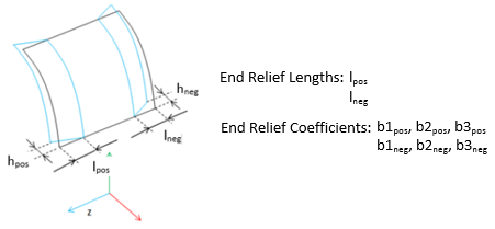 The end relief lengths (End Relief +ve Length) lpos and (End Relief -ve Length) lneg define the width, where the modification is applied. The end relief coefficients are dimensionless coefficients introduced to facilitate input for the end relief modifications. For each field, "End Relief +ve Coeff." and "End Relief -ve Coeff.", enter the three values b1, b2, b3 described below. 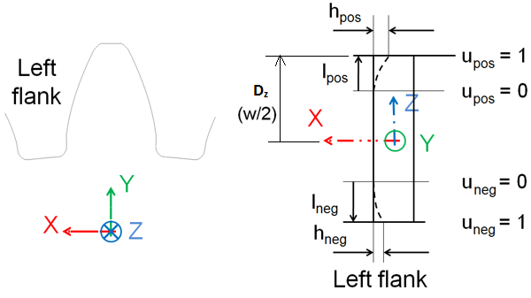 |
End Relief +ve Coeff. | |
End Relief -ve Length | |
End Relief -ve Coeff. | |
Following equations show the dimensionless variable upos and uneg. upos = ( Dz - ( gear_width/2 - lpos ) ) / lpos uneg = ( |Dz| - ( gear_width/2 - lneg ) ) / lneg where, Dz is distance from center to the end face of the gear measured along Z-axis as shown in figure. In correlation with crowning, a cubic polynomial from equations below defines the relief. hpos = b1pos * upos + b2pos * upos**2 + b3pos * upos**3 hneg = b1neg * uneg + b2neg * uneg**2 + b3neg * uneg**3 Equations below give the relation between the end reliefs hpos and hneg and a corresponding radius. Rpos = ( (lpos**2 + hcrown**2 ) / ( 2 * lpos ) Rneg = ( (lneg**2 + hcrown**2 ) / ( 2 * lneg ) Generally the relief is small compared to the length of the relief, what allows to approximate the radius by equations: b2pos = lpos ; b1pos = b3pos = 0.0 b2neg = lneg ; b1neg = b3neg = 0.0 Relief h1 at u = u1 ( u1 > 0.0 and u1 < 0.0) and h2 at u = 1.0 with no slope at u = 0 is defined by the coefficients of equations: b1 = 0 b2 = ( h1 - h2 * u1**3 ) / ( u1**2 - u1**3 ) b3 = ( h2 * u1**2 - h1 ) / ( u1**2 - u1**3 ) | |
Lead Slope | 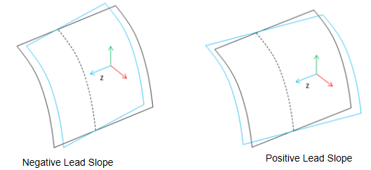 Lead Slope defines correction of the helix angle (), which is used to improve contact with mating gear teeth when system deflections would otherwise cause edge loading: 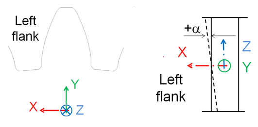 The principles for lead modifications are identical between left and right flank. The only point of attention is the definition of the lead slope as shown as: 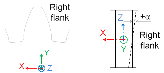 |
Mesh Properties Settings here that increase the size of the FE model can result in large temporary files in your working directory which can consume significant disk space (on the order of 1-50 GB). These include mesh density, number of contact planes and load element size. Note: Such settings can also significantly increase the time required to import the .cmd file representation of the model. Import times of several minutes can be experienced. This can be avoided by directly defining the gear part mass properties instead of basing them on a density and volume calculation (the volume calculation on fine shells is costly) | |
Mesh Density | Mesh density defines the number of finite elements along the contact line. 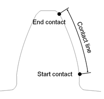 The contact line represents the portion of the profile (flank), where contact is supported. The contact line is defined through start contact and end contact: Start contact is close to the root for external and internal gears. Valid input entries for mesh density are 1 to 5, meaning 16,24,32,40 or 48 elements along the contact line. This input parameter allows the user to select his preference with respect of accuracy versus CPU-time. A low value for mesh density will result in a coarser Nastran model, what gives generally a short CPU-time. One has to keep in mind, that a coarse model is generally slightly stiffer. The Adams simulation time is not strongly influenced by mesh density. The pre-processing time, however, does increase noticeably with increases in mesh density. It is recommended that both meshing gears should have same mesh density. If unsure how to set this parameter, consider starting with 3 and increasing it if the results are not sufficiently accurate or decreasing it if they are sufficiently accurate and faster performance is desired. |
No. of Contact Planes | The integer value of number of contact planes divides the width of a tooth into a number of equidistant sections in lead direction. The number of elements across the gear width is equal to the "Number of Contact Planes" multiplied by the "Load Element Size". So, for example, if you have 10 contact planes and load element size = 2, then you get 10*2 = 20 FE elements along the tooth width. So, pre-processing time increases with increasing number of contact planes. It is recommended that the number of contact planes be the same on both gears in a pair. Contact between gear wheels is checked at each 'contact plane' of wheel 1 of the Advanced 3D Contact force. A too small number of contact planes may lead to some numerical noise. Adams simulation time increases with increasing number of contact planes. If unsure how to set this parameter, consider using the following formula to start with: u = width / ( 2 * module * 10 ) number contact planes = 20 * ( 1 - u ) + 30 * u Other advice: ■For spur gear or helical gears with helix angle < 8 degrees, the number of contact planes is mostly dependent on gear height: as tooth height increases the suggested number of contact planes decreases. Even for very narrow gears, avoid setting number of planes less than 10 without cautiously evaluating accuracy. ■For helical gears with larger helix angles (>=8 degrees) the value should be higher compared to the spur and low-angle helical gears. This helps to reduce the noise in results. For helical gears with a helix angle of 20 degrees we recommend roughly 30 to 50 contact planes, dependent on gear width (increase with increasing gear width, but at the expense of simulation time). |
Load Element Size | Load Element Size defines the number of finite elements in the lead direction per section. The number of elements across the gear width is equal to the "Number of Contact Planes" multiplied by the "Load Element Size". So, for example, if you have 10 contact planes and load element size = 2, then you get 10*2 = 20 FE elements along the tooth width. So, pre-processing time increases with increasing load element size.  With a value of 1 rough results can sometimes occur since the local deformation is coarse/averaged. If you are unsure what value to use, consider starting with the default value of 2 and then adjusting the number of contact planes to achieve the desired accuracy/run-time balance. |
Display Ratio Lead | The SHELLs are used for the display only; they are not used for any contact simulation. The input for Display Ratio Lead defines number of divisions for Shell geometry in lead direction as a fraction of contact planes number. Value 2 means half the number of divisions to the number of contact planes. 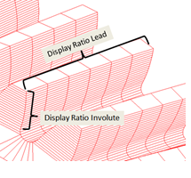 |
Display Ratio Involute | The SHELLs are used for the display only; they are not used for any contact simulation. The input for display ratio involute defines number of divisions for shell geometry in involute direction as a fraction of contact elements number defined by mesh density. Value 2 means half the number of divisions to the number of contact elements. |