Special Topics about the Adams Solver C++
This section provides another view of the Adams Solver C++ highlighting special features not found in Adams Solver FORTRAN.
Linearization
Linearization in the C++ solver is implemented using an exact algorithm that requires no numerical differencing. The linearization is exact in the sense that no simplifications are done on the equations of motion. All nonlinear effects of the motion (gyroscopic effects, Coriollis effects) due to velocities are taken into account exactly. The linearization can be done at any operating point.
Historical rules have been modified a bit. For example, when using the FORTRAN solver, the following simulation commands at time t=0:
simulate/statics
linear/eigensolution
will trigger the following behavior. First, after the statics simulation is finished (at time t=0), the velocities found in the *.adm file (the dataset file) will be restored. Second, the ongoing linearization command will reuse the Jacobian from the previous static simulation.
On the other hand, when using the C++ solver, the user has the option to stop restoring the velocities at time t=0. Moreover, the linearization does not reuse an old Jacobian but it will trigger a reconciliation if necessary. This reconciliation done by the C++ solver is required to bring the model to a consistent state. Typically, the reconciliation is done if the velocities were restored or if there were differential states having the STATIC_HOLD option.
Probably the main feature of the linearization in the C++ solver is the ability to linearize the system in terms of user defined states.
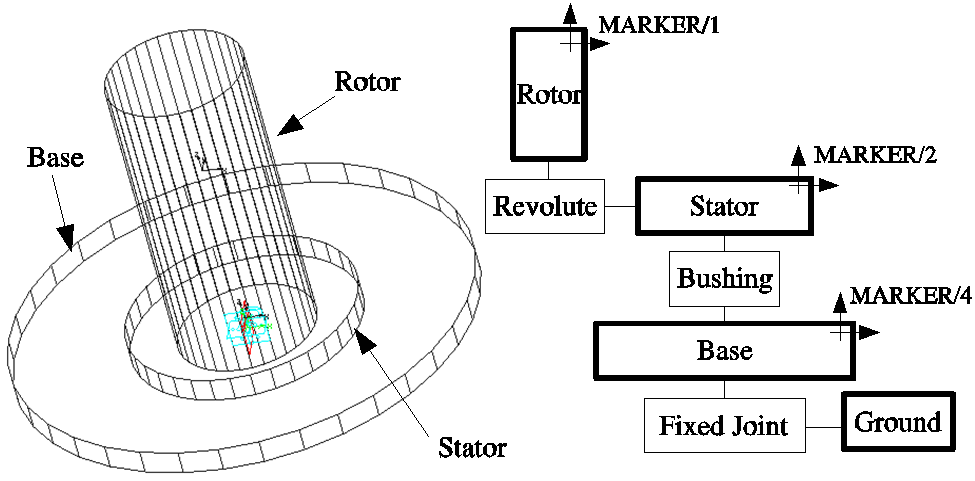
Figure 1 A rotor-stator model and topology diagram.
The model shown in Figure 1 is simple rotor-stator model where the Base object is fixed to GROUND. Figure 2 shows a plot of the eigenvalues versus the rotational speed of the rotor. The plot on the left was made using global linearization coordinates while the plot on the right was created using relative coordinates (using a PSTATE or RM options in the LINEAR command).
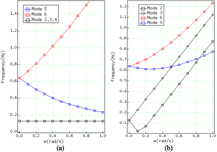
Figure 2 Eigenvalues versus rotational speed computed using global and relative coordinates.
While the values in Figure 2 can be verified either analytically or by building a physical prototype, a numerical approach is feasible by instrumenting the numerical model as shown in Figure 3 below.
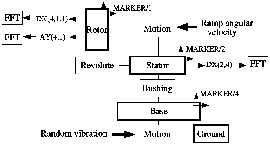
Figure 3 Instrumented numerical model
The instrumented numerical model is then subject to a dynamic simulation and the signals DX(4,1,1), AY(4,1) and DX(2,4) shown in Figure 3 can be obtained and post processed using an FFT tool.
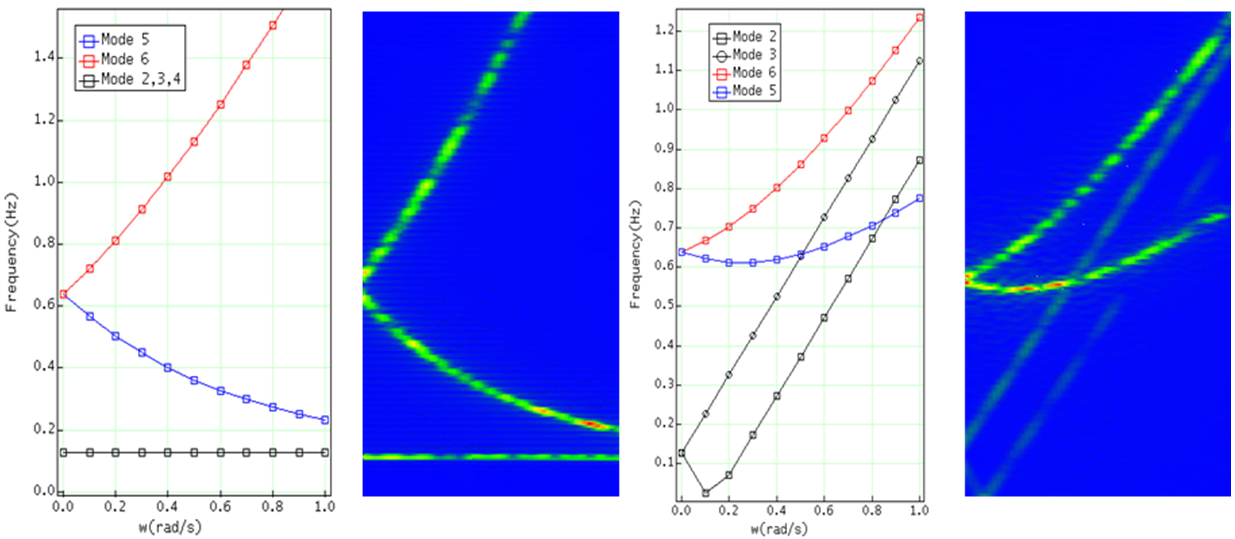
Figure 4 FFT plots compared with LINEAR results
Figure 4 shows the FFT results where an exact match between numerical and LINEAR results match.
Flexible Body Contact
Flexible body contact in the C++ solver implements a native flexible-to-flexible contact algorithm. There is no need to create MFORCE to model contact interactions. All the required information to handle the contact is obtained from the Modal Neutral File (MNF); this information includes the geometric information required to handle the geometry intersections.
The flexible-to-flexible contact implementation supports both solids and shell elements.
GCONs
The GCON statement in the C++ solver permits the creation of user-defined constraint equations. GCONs can be used to mimic standard joints or to create special constraint equations not supported by the MOTION, JOINT and JPRIM statements.
All the existing constraint objects in the C++ solver are implemented as GCONs. For example a SPHERICAL JOINT will create three GCONs equations automatically.
GCONs can be used to create non holonomic constraints.
CBKSUB
The CBKSUB (callback subroutine) was created for advanced users to help optimizing the execution of user-written subroutines. The CBKSUB is optional. If the user defines a CBKSUB, then Adams Solver C++ will call the provided subroutine at specified milestones during the code execution.
Milestones examples are: the end of reading the model, the start of an iteration, the start of a new time step, the end of a dynamic simulation, the shutdown process and so on.
The main feature of the CBKSUB is to allow the user have a clear control of the code execution in order to allocate memory in his/her user-written subroutines. Another important use of the CBKSUB is to use it as place to cache intermediate results.
The CBKSUB allows the user to make calls to SYSFNC and SYSARY subroutines without creating dependencies.
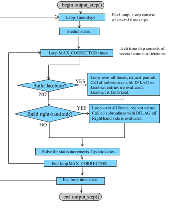
Figure 5 Architecture without CBKSUB.
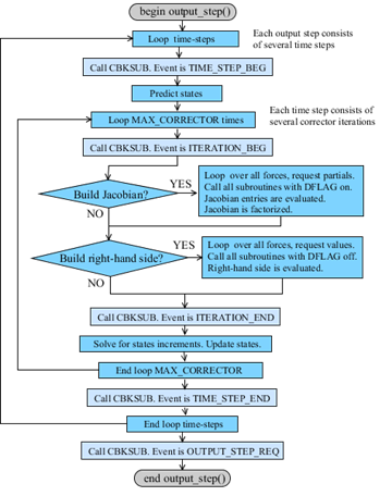
Figure 6 Architecture with the CBKSUB.
Notice that Figure 5 and Figure 6 show a simplified version of the Adams Solver code. Also, not all milestones are shown. Profiling tests show that the overhead of calling the CBKSUB is negligible.
Adams-to-Nastran Export
The Adams-to-Nastran utility is available under the LINEAR command. The tool generates and exports a fully editable Nastran data deck equivalent to the Adams model. Figure 7 below shows such a translation.

Figure 7 Adams-to-Nastran example
The Nastran model shown on the right of Figure 7 is created automatically and it is ready for a SOL107 solution in Nastran. Tests show eigenvalues computed by Nastran and Adams match surprisingly well (see Figure 8 below).
Figure 8 Eigenvalues comparison Adams versus Nastran.
In general, Adams-to-Nastran export can save considerable man power when chain simulations are required.
FE_PART
Starting version Adams 2014, Adams Solver C++ implements natively (fully implemented in Adams) finite elements with distributed mass. Some of the main features of this element are:
1. Elements use ANCF technology mixed with Timoshenko beam theory.
2. Geometrically large displacements are supported.
3. Contact support.
4. Allows user to put MARKERs on the elements and attach forces or constraints.
5. Full pre and post processing support
6. Curve isoparametric formulation.
7. Variable twisting cross section properties.
8. Support for defining distributed loads.
9. Linear material implementation supporting elastic, orthotropic and anisotropic options.
Running Multiple Solver Batch Runs on Windows
The following steps will allow you to run multiple solver runs on a Windows server.
1. Create an .acf and .adm file for each model to be run. This can be done in one of two ways after a model and simulation script has been created:
a. Using the Write Files Only setting in Simulation Settings panel for the Executable option.
b. Set the Solver Settings to Output with Save Files set to Yes with a File Prefix defined.
Example "test_1.acf" file for "test_1" simulation script:
2. Create a batch file (batch_run.bat) for all the models to be run as follows:
Note: | The Adams version environment variable here is adams2020 with existing models "test_1", "test_2", and "test_3". |
3. Run the bat file from the Adams Command Prompt window by invoking it with this command:
> batch_run.bat
Note: | This method makes sure that all other models will run even if one of the models fails. |
High Performance Computing
The C++ solver has a set of subsystems implementing High Performance Computing (HPC) using multithreading (SMP). The multithreading code is written using the Pthreads API (POSIX). Among the parallelized subsystem there is the parallel Jacobian evaluation, parallel linear algebra and parallel results generation. Other subsystem use threading pools for other chores.
Thread Affinity Settings in Adams
Overview
There is no consensus on a standard nomenclature regarding hardware components found in common desktop computers used in research and engineering. Therefore, in this section, terms like CPU, PU, core, socket, node, logical CPU, will follow the nomenclature used by the Portable Hardware Locality (hwloc) software package [1].
This section will cover a diverse set of subjects like hardware architecture, operating system scheduler, thread affinity, sockets, hyperthreading and so on, all of which are required in order to make the best decision regarding affinity settings for a simulation job. Brief notes on thread priorities are also included.
Since 2005, Adams Solver C++ supports the PREFERENCES/NTHREAD option to define the number of parallel threads (multithreading) to be used for the numerical simulations. Multithreading algorithms were designed and implemented to execute diverse tasks like the assembly of the equations, matrix manipulations, asynchronous output and so on. However, Adams Solver C++ relied completely on the operating system's scheduler for the thread affinities. Thread affinity is defined as the location (the CPU) where the thread is running. The operating system's scheduler is a module that has the task of assigning the affinity of all running threads in the machine. (Among other chores, the scheduler decides which thread runs when.)
By default, if there is no software or user intervention, the OS scheduler will completely determine the affinity of a running thread. Notice the affinity may be a single CPU or it may be a set of CPUs (an affinity set); moreover, the thread's actual affinity may be changing in time. The scheduler is free to change the location of a thread at any time. Notice most operating systems do provide tools for the user to intervene and define the affinity set of a running application. See, for example, the taskset command in linux. If there is intervention, the scheduler will confine a thread to a single CPU or to a defined set of CPUs depending on the commands issued by the user.
Regardless whether there was user intervention or not, the affinity of each thread will in general depend on the whims of the scheduler (the actual algorithm used by the OS), the load on the machine (for example, network traffic), and the thread priority.
The thread priority can be one of two main types: normal priority and real time priority. All operating systems provide variations of those two main types. If there is no intervention, all applications and their running threads will run using a default priority managed by the operating system. Some applications, for example, Simulation Workbench ®[2], run using real time priorities, and they do launch other applications (for example, Adams Solver C++) with real time priorities as well. Users need nothing to do regarding thread priorities when using Adams Solver C++ in real time simulations and in most standard cases.
Adams Solver C++ does not provide tools to set the priority of its threads. You may, however, run Adams Solver C++ using real time priorities in any standard computer environment provided you have the permissions and the operating system support. For example, see the chrt command in linux for more details.
Adams Solver C++ does provide a way to define the affinity set for the Adams process via an environment variable or FMU fixed parameter. It requires a basic knowledge of the machine architecture and some basic concepts of the operating system. More details on these are found later in this section. Using this variable or parameter, Adams Solver C++ will intervene at the software level to modify the affinity of its threads.
Hyperthreading and Logical CPUs
Before circa 2001, desktop computers had only one Central Processing Unit (CPU) and the terms CPU and core were used interchangeably. Figure 9 shows a basic diagram of a CPU at that time. The Arithmetic Logic Unit (ALU) and the Registers interact with the Bus interface that connects the CPU with the rest of the computer, for example, the memory.
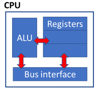
Figure 9 Before circa 2001. CPU and core are synonyms.
Although desktop computers at that time were equipped with a single CPU, multithreading was already enabled and popular. Graphical interfaces were already blooming due to the operating system's capability to support multiple execution threads. The job of the scheduler was to manage all running threads to provide them with a time allocation to run on the single available resource. However, around 2001, a new chip design allowed a CPU to have two sets of Registers sharing the same ALU as shown in Figure 10. Using this new technology, two threads (or processes) could be running almost independently provided one thread was not using the ALU.
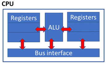
Figure 10 Hyperthreading enabled chip (circa 2001).
Notice however, the performance of hyperthreading is small or negligible for heavy computational tasks that require frequent use of the ALU, for example, numerical simulations. For other types of applications, hyperthreading does provide a clear performance gain, for example, graphical interfaces.
Hyperthreading required the creation of the term logical CPU. A logical CPU, a.k.a. Processor Unit (PU), is the current definition used to refer to an execution capable unit. A logical CPU is the smallest entity that can run an execution thread. Besides the creation of the term logical CPU (or PU), the term core was redefined as a set of either 1 or 2 logical CPUs, depending whether hyperthreading is enabled or not. Figure 11 shows a core with hyperthreading enabled. Notice logical CPUs started to be numbered.
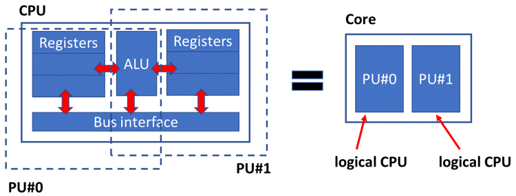
Figure 11 Logical CPU or PU.
Users should keep in mind that hyperthreading is a configurable feature. A hyperthreading capable computer can be re-configured (at the BIOS level) to disable the hyperthreading capability.
Multicore Machines
Around circa 2002, new desktop computers began to include several cores (multicore machines). Suitably, the term socket was introduced to mean a set of cores. The term core continued to define a set of 1 or 2 logical CPUs. Cores started to be numbered as well. Figure 12 shows on the left the case of a multicore machine with 4 cores and hyperthreading enabled; on the right we observe the case of machine with hyperthreading disabled.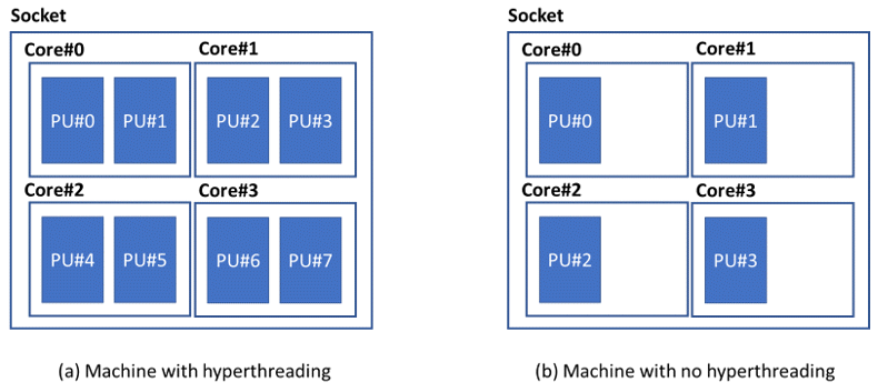
Figure 12 Two multicore machines.
There are two important facts to remember. The first one is that operating system tools use the term CPU to mean logical CPUs. Second, the logical numbering of the CPUs (for example, PU#0, PU#1 and so on) is completely arbitrary and depends on both the OS and the BIOS. For example, Figure 13 shows a computer that has PU#0 and PU#1 not located on the same core; compare it with the computer shown in Figure 12 (a) which has PU#0 and PU#1 located on the same core.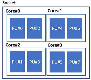
Figure 13 Logical CPUs have arbitrary numbering.
The arbitrary numbering of logical CPUs is of outmost importance when selecting the affinity set to run Adams Solver C++. For example, assuming the user runs Adams Solver C++ with 4 threads using the machine shown in Figure 12 (a), an optimal affinity set would be "0, 2, 4, 6". That selection guarantees that only one thread runs per core. Running the same model on the machine shown in Figure 13, an optimal set would be "0, 1, 4, 5". Clearly, the arbitrary numbering of logical CPUs is not an issue if hyperthreading is disabled. See next section for other issues related to affinity sets in machines with multiple sockets.
The fact that hyperthreading is not beneficial for heavy computational tasks, can also be observed when using third party tools like the Intel MKL Pardiso (numerical algebra solver tool) [3]. Pardiso will ignore hyperthreading and will cap the number of threads to the number of cores.
NUMA Controllers
Following a natural progression, after circa 2002, multi socket computers were introduced in the market. Figure 14 shows one such a computer having two sockets. Sockets started to be numbered. Each socket has a NUMA controller (a.k.a. NUMA node). NUMA controllers are the interface of each socket with the main memory of the machine.
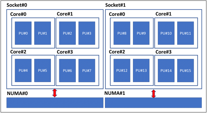
Figure 14 A machine with 2 sockets, 4 cores per socket and hyperthreading enabled.
A most important fact for users is that threads have lower latency accessing memory data managed by the corresponding NUMA node than accessing memory data managed by another NUMA node. For example, referring to Figure 14, a thread running on PU#6 will get a faster response for memory allocated by NUMA#0 than for memory allocated by NUMA#1. Therefore, the optimal affinity set for Adams Solver C++ is a set of logical CPUs belonging to the same NUMA node.
Recapitulating, affinity settings allow users to define the set of logical CPUs where the Adams Solver C++ will run its threads. For optimal performance, that set must be carefully defined to have one logical CPU per core, and the set must belong to the same socket. You still may define additional CPUs from other sockets, but the performance gain may not be as expected.
Moreover, not all sockets run equally fast. Other third-party software vendors have confirmed this same observation: running a process in one socket may be 3% slower than running the same process in another socket. A possible explanation is the asymmetry of the hardware or that the load of the operating system favors one socket more than the other.
Tools to Examine Hardware Topology
All operating systems offer tools to examine the machine's topology. For example, the command lscpu in linux Red Hat 7.3 prints a report as shown in Figure 15.
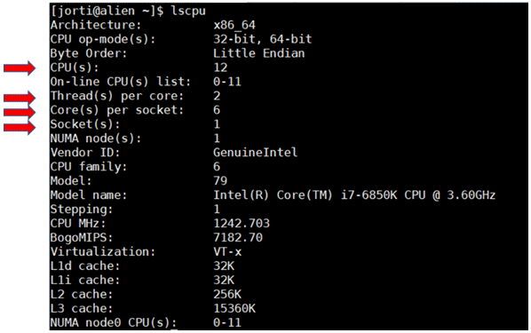
Figure 15 Tools to examine the hardware topology
Here, CPU(s) stand for the number of logical CPUs. The number of logical CPUs per core is reported as Thread(s) per core because it is equivalent to the number of threads that can be run on one core. Accordingly, the value is either 1 or 2. If the value is 2, hyperthreading is enabled. The command also displays the number of cores per socket and the number of sockets in the machine.
The Portable Hardware Locality (hwloc) is a free tool including utilities that can display the machine's topology in a graphical form (hwloc comes included in some linux distributions). Figure 16 shows the graphical output of hwloc's lstopo on a small Windows laptop. Notice the machine has 1 socket, 4 cores per socket, and 2 logical CPUs per core (hyperthreading enabled). The operating system of this machine reports a total of 8 CPUs (logical CPUs).
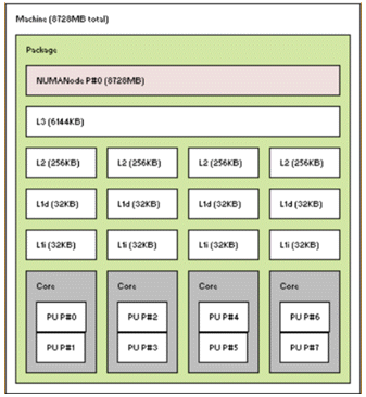
Figure 16 lstopo output for a small laptop computer.
Figure 17 shows the lstopo graphical output on a small linux desktop computer. That computer has 2 sockets, 6 cores per socket, and 1 logical CPU per core (hyperthreading disabled). The operating system of this machine reports a total of 12 CPUs (logical CPUs).
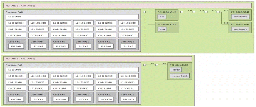
Figure 17 lstopo output for a small desktop computer.
Figure 17 also shows an interesting fact: some cores may be disabled. Notice cores 1-5 and 7-8 are not displayed in the topology view of the machine. Regardless of disabled cores, the numbering of the logical CPUs is always consecutive and starting at zero.
Terminology and Important Facts for Adams Affinity Settings
Setting the affinity for Adams Solver C++ requires the user to know the basis of hardware topology and to have a basic understanding of the role of the operating system. To help in that regard, Table 1 below lists basic terminology used in this document.
Table 1 Useful hardware and OS terminology
Term | Definition |
|---|---|
Computer | As set on NUMA nodes (or sockets) |
NUMA node | Memory controller for a socket |
Socket | A set of cores |
Core | A set of 1 or 2 logical CPUs. A core has 1 Arithmetic Logic Unit (ALU) and 2 Processing Units (PUs). See Figure 11. |
Logical CPU | Smallest processing unit (PU) capable to run a thread of execution. Operating systems call them just CPUs. |
Hyperthreading | Configurable feature to run two execution threads in a single core. |
Scheduler | Operating system module in charge of determining when a thread (or process) runs, and where it runs. |
Affinity | The logical CPU where a thread (or process) runs. If there is no user intervention, the affinity of a thread may change at run time at the whims of the scheduler. |
Affinity set | A set of logical CPUs. Adams Solver C++ allows users to define a set of logical CPUs for the process. The operating system provides tools to set the affinity. |
Table 2 lists a set of important facts related to affinity settings.
Table 2 Useful facts regarding affinity settings
Context | Important fact |
|---|---|
Hyperthreading | It is configurable, it can be disabled at the hardware level. |
Hyperthreading | Provides a performance boost in many cases except in heavy numerical computations. |
Affinity set | For optimal performance, if hyperthreading is enabled, select one logical CPU per core. |
Affinity set | For optimal performance, the logical CPUs must belong to the same socket. |
Affinity set | You may select logical CPUs from different sockets, but performance would not be as good as if all CPUs belong to the same socket. |
Affinity set | All logical CPUs are numbered consecutively starting at zero. Numbering of physical units is arbitrary. |
Socket | Running a process in one socket may be slower than running the same process in another socket. |
Socket | Some sockets may have disabled cores. |
Affinity Settings in FMI Real Time Environments
FMI real time environments are becoming the default standard for users to run real time simulations. Adams Solver C++ allows creating FMU models to run in FMI real time environments like Simulation Workbench [3] or SCALEXIO [4]. Real time environments have restrictions on CPU usage hence there is the requirement to set the affinity of running processes.
Given that real time environments make exclusive use of some logical CPUs for the OS to work, it is the user's responsibility to setup the affinity set for each running application in such a way that reserved CPUs are not used by his/her applications.
Given that the running Adams FMUs are launched by the real time environment, there is no practical way to use the operating system commands to define the affinity set of the Adams process. To overcome this issue, the Adams FMU has an FMU parameter named thread_affinity_set0 that can be used to set the affinity set for the Adams FMU. The value for this parameter is two integers separated by a hyphen. In other words, we can only define a consecutive set of CPUs. Fortunately, most of real time environments have hyperthreading disabled.
As an alternative, you may define the affinity set for the Adams FMU using an environment variable. The format (name and value) are as follows:
Name: MSC_ADAMS_THREAD_AFFINITY_SET0
Value: A comma separated list of CPU numbers or ranges (two digits separated by a hyphen)
Example (linux):
%> setenv MSC_ADAMS_THREAD_AFFINITY_SET0 "1, 2, 5-6"
Instead of using the OS to set the environment variable, you may use the ENVIRONMENT statement in your Adams data set as follows.
Example:
ENVIRONMENT/NAME=MSC_ADAMS_THREAD_AFFINITY_SET0, VALUE="1, 2, 0-5"
In real time environments the size of the affinity set (the number of logical CPUs listed) must match the number of threads being set for the model (for example, PREFERENCES/NTHREAD). If the size of the set is smaller than the number of threads, Adams Solver will place more than one thread on the same CPUs affecting performance. If the size of the affinity set is smaller than the number of threads, the CPUs with larger index will be ignored.
Affinity Settings in Standard Environments
Regarding thread priorities, operating systems do allow a superuser to run applications with real time priorities in standard laptops, desktops, and servers. One advantage of using real time priorities is that the process will run uninterrupted. Adams Solver C++ does not provide tools to launch an Adams process using real time priorities. For that endeavor, users ought to use the operating system tools. An additional boost may be obtained using the concept of shielding. Consult the operating system documentation for more information on shielding.
Regarding affinity settings, most of the time there is no need to set the affinity set for an Adams simulation running in a standard setting. If the machine is not heavily loaded with multiple applications running at the same time, the scheduler will be smart enough to provide performance with multithreading, even in case of running multiple Adams jobs at the same time.
However, not all schedulers are equally smart. We have observed the scheduler in some SUSE distribution to cluster all the threads of multiple Adams jobs on a small set of CPUs. The solution to this issue was to launch each Adams job with a different affinity setting. This way, the performance of running multiple Adams jobs on the same machine was comparable as the performance of running a single Adams job. The most practical solution is to modify the scripts that launch the jobs using the operating system commands.
Caution: | You may need to set affinities for multiple Adams job running at the same time on the same computer. |
Option ALL
The environment variable MSC_ADAMS_THREAD_AFFINITY_SET0 has an additional option ALL that will set the affinity of Adams threads in a one-to-all fashion. By default, the affinity settings are one-to-one as shown in Figure 18. In the default case, each thread is assigned a single CPU from the set. In this case, the scheduler will bind each thread to a unique CPU.
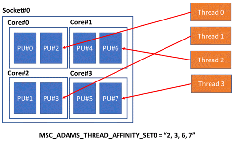
Figure 18 Default affinity settings, one-to-one.
Alternatively, using the ALL option, the affinity for each thread is set using a one-to-all fashion, as shown in Figure 19. In this case, Adams Solver C++ will assign the complete set of CPUs for each thread. The scheduler will be allowed to run each thread on any of the CPUs in the set.
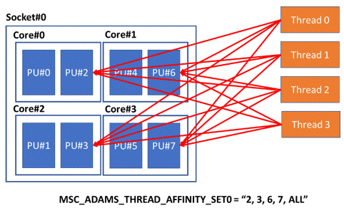
Figure 19 Using option ALL, one-to-all.
Option ALL may provide additional performance gains in some architectures, or in cases when the number of threads is larger than the size of the affinity set.
References
1. Portable Hardware Locality. https://www.open-mpi.org/projects/hwloc/
2. Simulation Workbench. https://www.concurrent-rt.com/products/simulation-workbench/
3. Intel MKL Pardiso. https://software.intel.com/en-us/node/470282
4. Scalexio. https://www.dspace.com/en/inc/home.cfm