The MFORCE statement applies a force directly to the modal coordinates and rigid-body degrees of freedom of a FLEX_BODY.

The MFORCE statement allows you to apply any distributed load vector F to a FLEX_BODY. Such a load vector is typically generated with a finite-element program. Examples of distributed loadcases include thermal expansion or pressure loads. To help you understand how Adams handles distributed loads, the following section discusses the equations of motion of a flexible body, starting with the physical coordinate form that the finite-element program uses.

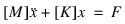
where and are the finite element mass and stiffness matrices for the flexible component; x is the nodal coordinate vector; and F is the distributed load vector. This equation can be transformed into the modal coordinates, q:

where is the matrix of mode shapes. The modal form simplifies to: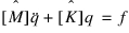

where and are the generalized mass and stiffness matrices, and f is a modal load case vector that Adams uses to define the MFORCE element.

The projection of the nodal force vector on the modal coordinates:

This is a computationally expensive operation that poses a problem when F is a general function of time. Adams circumvents this problem by assuming that the spatial dependency and time dependency can be separated such that the load is a time varying linear combination of an arbitrary number of static loadcases:

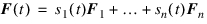
Therefore, the expensive projection of the load to modal coordinates is performed only once during the creation of the MNF, rather than repeatedly during the Adams simulation. Adams needs only to account for the modal form of the load:

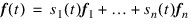
where the vectors f1 to fn are n different loadcase vectors. Each of the loadcase vectors contains one entry for each selected mode.

A more general definition of f allows it to have an explicit dependency on system response, which is denoted as f(q,t), where q represents all the states of the system. The equation for the modal load is then:

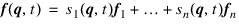
which allows the load on a flexible body to be a function of its proximity to another body, such as a heat source, its velocity, or other.

Adams Solver (FORTRAN) lets you define a modal load with the general definition in the last equation. However, because of the definition’s comprehensiveness, you may find it cumbersome to use. Depending on your needs, you may be able to use one of the more elementary versions, which are described next, beginning with the simplest definition.

If the FLEX_BODY receiving the load has the modal loadcases f1, f2,...,fn defined in its MNF, you can define the MFORCE by referring to exactly one of the loadcases using the CASE_INDEX argument. The loadcase is scaled using the SCALE argument, making the load a function of time and/or system response. This corresponds to the load definition:

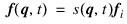
where CASE_INDEX=i and SCALE=s(q,t) is expressed as an Adams Solver (FORTRAN) function expression.

Alternatively, you can achieve the same effect using the MFOSUB user-written subroutine. The MFOSUB references one of the loadcases and computes the scale factor:

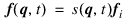
where the dependency on q occurs through the use of SYSFNC or SYSARY in the user subroutine. This method of MFORCE definition is strictly equivalent to the first one.

Alternatively, you can use MFOSUB to combine the loadcases, f1,...,fn as follows:

In this case, rather than referencing a single loadcase, the MFOSUB computes a new loadcase by combining the existing loadcases in a time varying fashion. Adams Solver (FORTRAN) then scales the new loadcase by a scale factor that is also computed by the MFOSUB. It is important to note that although the scale factor can be a function of time and of system state, the new loadcase may be only a function of time. In other words, using values obtained by calls to SYSFNC or SYSARY to define the functions gi(t) is not allowed.

If the FLEX_BODY has no loadcases in the MNF, then MFOSUB can compute the loadcase. Again, the loadcase vector may be a function of time only, while the scale factor that is applied to it may be a function of both time and system state:

where s(q,t) is a user-defined scale factor and fu(t) is a user-defined load vector. This method of MFORCE specification is primarily provided for completeness, and will be used primarily by very experienced users.

The general force description:

where each loadcase fi has its own response-dependent scale factor si(q,t) that can be achieved only through the use of multiple MFORCE elements acting on the same flexible body.

Definition 6:

This is expanded definition of Definition 3 to allow you to indicate multiple scale factors. The force description is same as Definition 3 as follows:

The values of e(q,t) and g1(t), g2(t), … gn(t) are specified in MFOSUB instead of e(q,t) and the term of [ ] in Definition 3. Note that the modeling is quite same as Definition 3 but this is useful for correct MFORCE visualization in Adams PostProcessor.

For distributed loads that have an external resultant, portions of the load will project on the rigid body modes of the flexible body. However, the rigid-body modes must be disabled because Adams Solver (FORTRAN) will replace them with the nonlinear, large motion, generalized coordinates: X, Y, Z, , , and . In this case, the load on the rigid-body modes are transferred to the large motion generalized coordinates.

Part of this transfer occurs during the MNF2MTX translation of the flexible body's MNF, and, consequently, the MODLOAD matrix has a dimension that equals 6 plus the number of modes. The first 6 entries in each column correspond to the external force and torque acting on the flexible body for this loadcase, expressed relative to the body coordinate system (BCS). When the loadcase is an internal force (as would be expected in the case of a thermal load), this force and torque will be zero.

You should also be aware of the way modal truncation affects the application of modal load. When you define a distributed load, it will be projected on the available modes. It is important to understand that the available modes form an efficient but incomplete basis for the flexible component. Therefore, it is inevitable that some portion of the load will be orthogonal to modal basis. This portion of the load will be irretrievably lost. Furthermore, during mode selection within Adams, you should realize that a mode whose removal is being considered may also have a significant modal load associated with it. In this case, the mode should not be disabled.

Using the first loadcase defined for FLEX_BODY/1, this example defines a modal load on FLEX_BODY/1 by scaling the values of the loadcase by the function expression SIN(TIME)*DX(1,4). The reaction force that corresponds to this load is ignored.

This example defines a modal load whose reaction resultant force acts on the parent part of floating marker 2. The magnitude and shape of the load is provided by the MFOSUB user-written subroutine, based on the user parameters 10,1e5,23.

See other Forces available.