Steps for Running the Example
1. Ensure you have an installation of Actran 2020 SP1 or later
2. Copy the tutorial directory included with the installation from "<top_dir>\acoustics\examples\tutorial\tuning_fork\" to some location on your machine you are comfortable using as a working directory
Note: | "top_dir" is the path in which Adams was installed. |
3. Launch Adams View, choose to open an existing model and browse for tuning_fork.cmd in the directory to which you copied it.
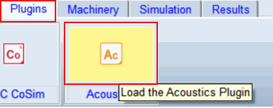
4. On the Plugins tab of the ribbon inside the Acoustics container, click the Actran logo to load the plugin:
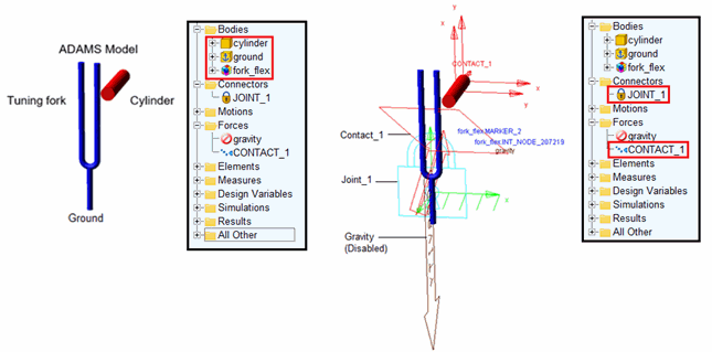
5. The model should now be open in the Adams View session. Familiarize yourself with it. It consists of a tuning fork flexible body, "fork_flex," and rigid body "cylinder" part that has an initial velocity in order to strike the tuning fork. The tuning fork is fixed to ground and there is a contact force between it and the cylinder. Gravity is disabled.
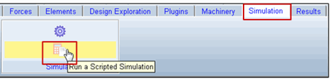
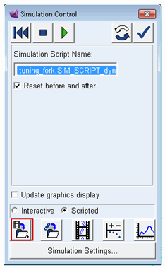
6. Simulate the Adams model:
a. Go to the Simulation tab
b. Click on the button Run a Scripted Simulation
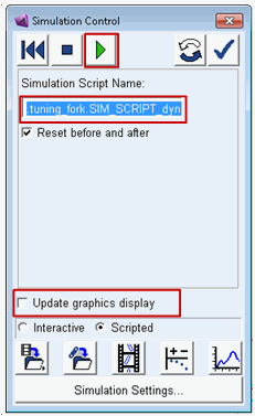
c. Enter the Script Name ".tuning_fork.SIM_SCRIPT_dynamic_run"
d. Uncheck Update graphics display
e. Start the Simulation
f. The simulation is performed with a time step  up to
up to 
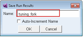
up to 7. Save the simulation
a. Click the button shown below to save the results under a named analysis object
b. Save the results under the name "tuning_fork"
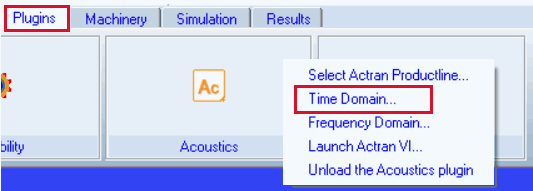
8. From the Plugins tab on the ribbon go to the Acoustics container, click the Actran logo and select Time Domain to launch the dialog to setup and run the Actran analysis.
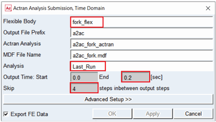
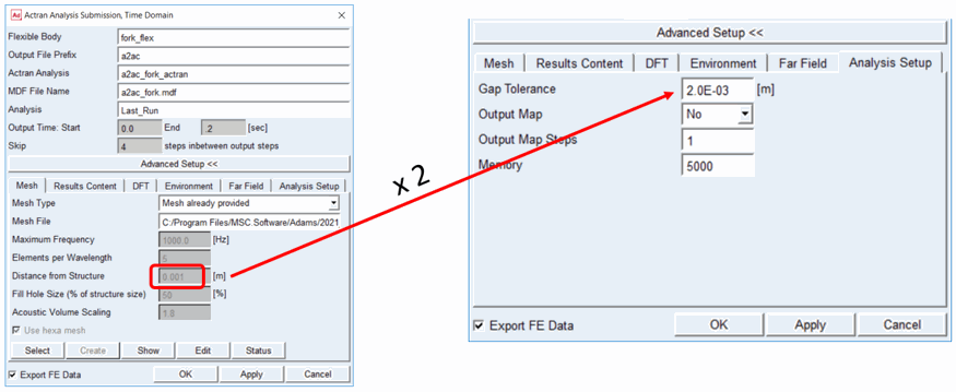
9. Fill out the main area of the dialog as shown below, but do NOT click OK/Apply yet because we want to specify some Advanced Settings Next:
a. Choose "fork_flex" as Flexible Body
b. Use "Last_run" as Analysis
c. Compute the simulation up to 0.2sec
d. Skip 4 steps in-between the Adams output steps, thus the Actran output step is set to 5e-4sec
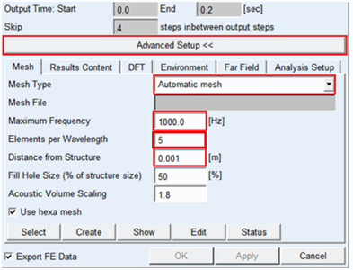
10. Click on Advanced Setup and make the following selections on the Mesh tab
a. Set Mesh Type to Automatic mesh
b. Based on Time step and the entry for Skip above, set Maximum Frequency of 1000.0 [Hz] is good proposal
c. Set Elements per Wavelength to 5
d. Distance from Structure: choose 0.001m
e. Click the Create button
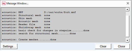
11. The mesh creation is complete when the following information is displayed:
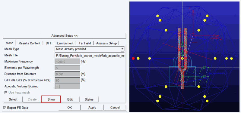
12. Click on the Show button
a. The generated Acoustic Mesh is displayed
b. 40 Microphone locations are shown as yellow spheres
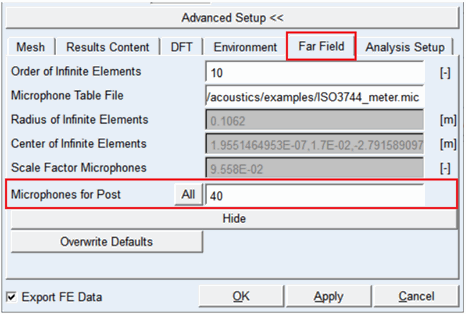
13. Go to the Far Field tab to select at which microphone locations results should be generated
a. The "All" button will display all microphones
b. In the Microphones for Post field specify 40, which is selected by default
c. The sphere representing the selected microphone(s) will be colored red instead of yellow
14. On the Analysis Setup tab set Gap Tolerance to 2.0e-3 m. Typically, Gap Tolerance should be twice the value of "Distance from Structure" on the Mesh tab.
15. Go to the DFT tab to setup the Discrete Fourier Transformation
a. Use a Time Interval of 0.1s (window length of DFT)
b. Set Overlap of Time Interval = 0%
c. Set End Frequency = 1000.0 Hz. This value is derived based on the length of the simulation time steps ( ) and then via the Nyqvist criterium the maximal computed frequency becomes
 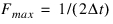 = 1000 Hz.
) and then via the Nyqvist criterium the maximal computed frequency becomes = 1000 Hz.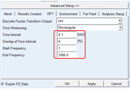
16. Launch the Acoustic analysis by clicking the OK button.
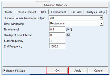
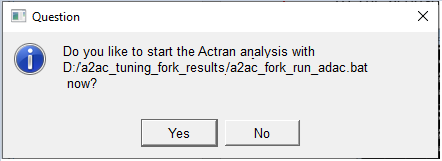
17. Choose Yes to start Actran analysis
■You can select No if you want to edit the parameter file (a2ac_fork_actran.par) and submit the analysis manually.
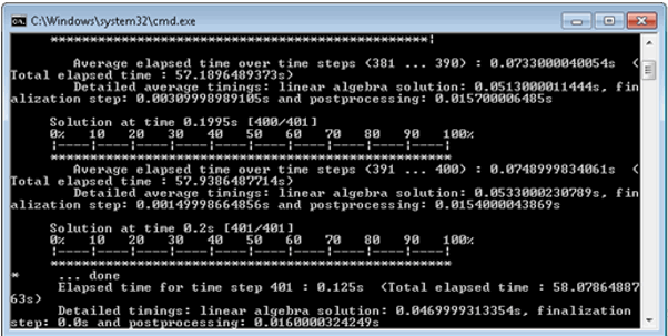
18. The acoustic analysis progress is displayed in a separate window:
19. When the acoustics analysis is complete you will notice that in the working directory a new directory "a2ac_Last_Run_results" is created containing the acoustic Actran model, input files and post-processed results. (Separate directories will be created for each acoustics analysis)
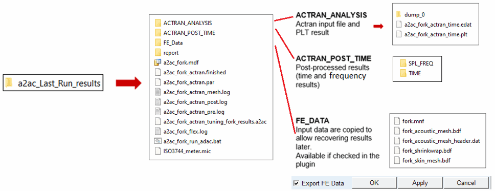
20. The time dependent results (ACTRAN_POST_TIME / TIME) are stored as images in the working directory:
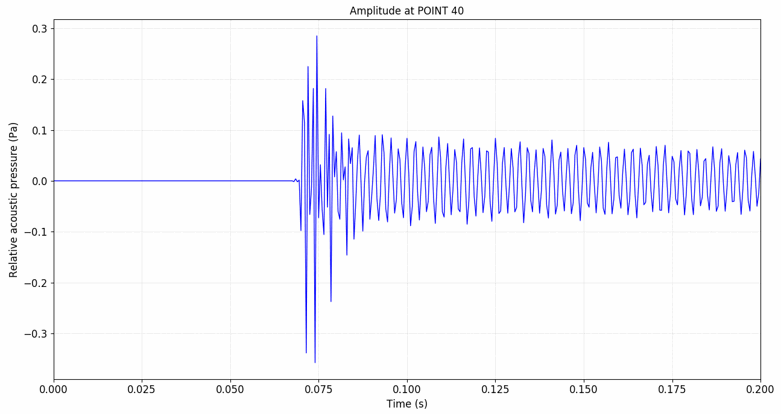
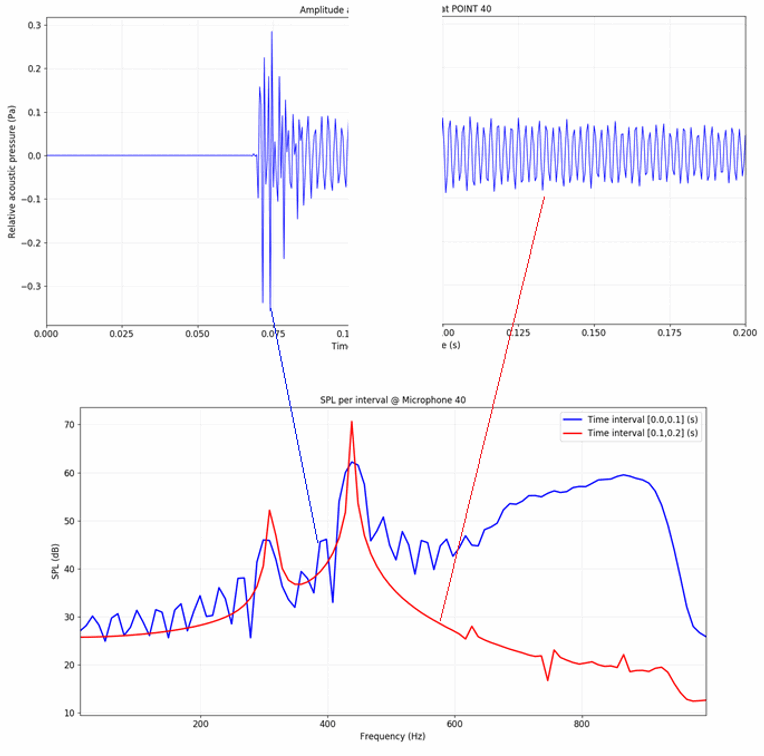
a. Transient results of microphone one ("a2ac_fork_sound_POINT_40.png")
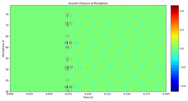
b. Transient results of all microphones ("a2ac_fork_Waterfall_Pa_all_microphones.png")
21. The frequency dependent results (Results ACTRAN_POST_TIME / SPL_FREQ) based on the settings that were entered on the DFT tab are stored as images in the working directory
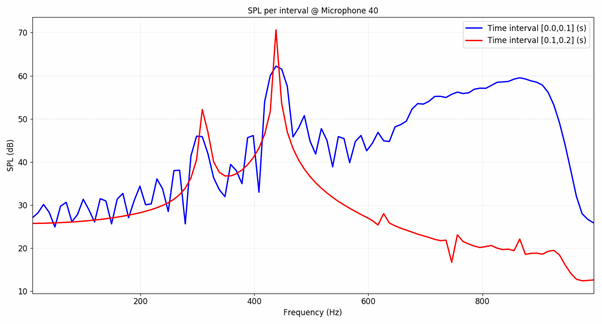
c. DFT of two time intervals ("a2ac_fork_actran_micros_pa_40_DFT_dB.png")
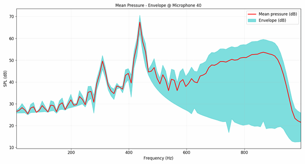
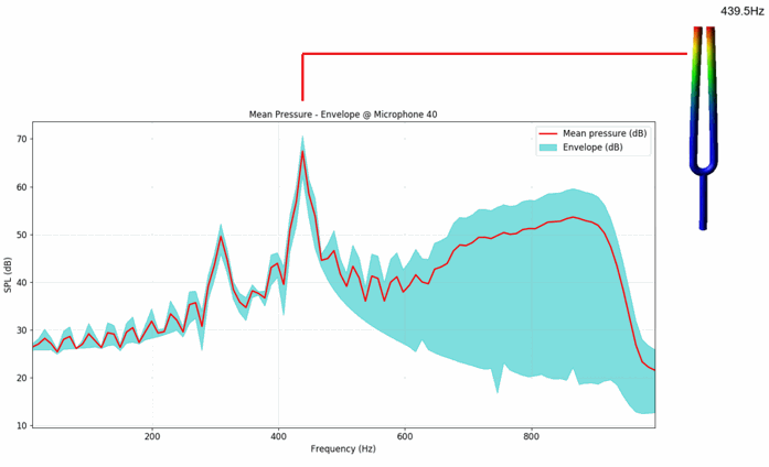
d. Envelope and mean values of both intervals ("a2ac_fork_actran_micros_pa_40_DFT_MeanPressure_Envelope_dB.png")
22. Notice that the time results are split in two parts
a. The DFT of the first part (0.0s-0.1s) contains the time period without excitation
b. The frequency content of this signal is relatively broad
c. The second part (0.1s-0.2s) contains the steady state response with a peak at 440Hz which represents the mode at 440Hz of the tuning fork
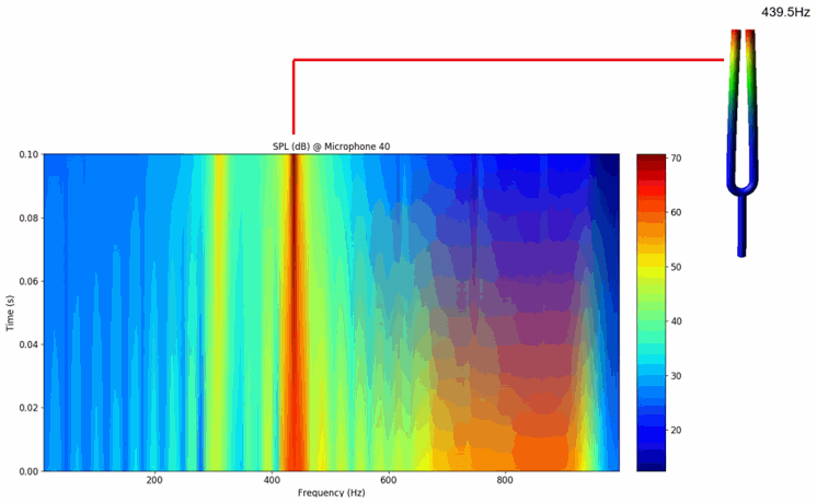
23. The frequency content of the time signals is output in file "a2ac_fork_actran_micros_pa_40_DFT_waterfall_dB.png" and you will notice that the first mode of the tuning fork flexible body is driving the acoustic radiation.
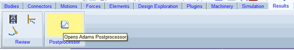
24. To plot results within Adams, switch to the Adams PostProcessor window:
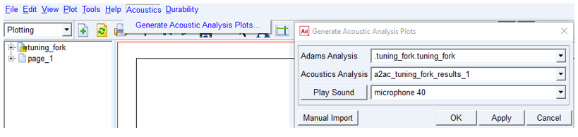
25. From the Acoustics menu select Generate Acoustic Analysis Plots and choose the Adams analysis and Acoustics analysis run in this exercise and click OK.
a. Note that it is posisble to run multiple acoustics analyses per a single Adams analysis as illustrated below
b. The Manual Import button can be used to import acoustics results manually (for example, if you have results from an Acoustics toolkit installation that pre-date the product plugin release)
26. Auto-Plotted Results:
a. Transient results of each Microphone in a 3D plot
b. Frequency dependent results over the time period
c. Sound pressure level at each time interval
d. Mean pressure
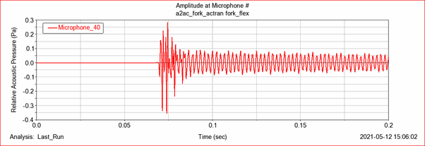
e. Amplitude
f. Overall Sound Pressure Level (OSPL) per time step
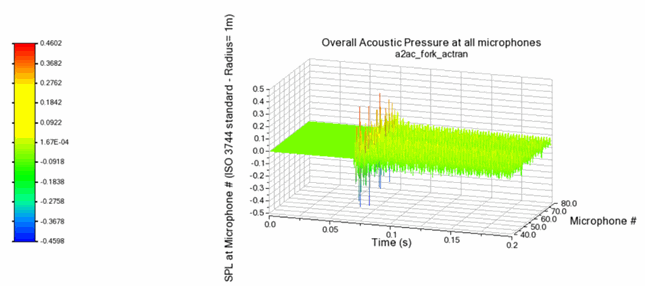
a. Transient sound pressure level at all microphones
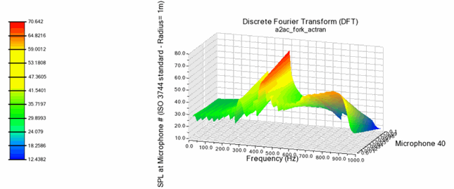
b. Frequency dependent results at all microphones
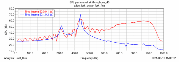
c. Sound pressure level at each time interval
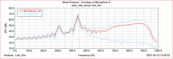
d. Mean pressure
e. Acoustic amplitude
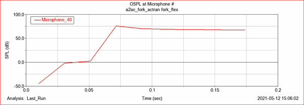
f. Overall sound pressure level