Steps for Running the Example
1. Ensure you have an installation of Actran 2021 or later
2. Copy the tutorial directory included with the installation from "<top_dir>\acoustics\examples\tutorial\Tuning_Fork_Adv\" to some location on your machine you are comfortable using as a working directory
Note: | "top_dir" is the path in which Adams was installed. |
3. Launch Adams View, choose to open an existing model and browse for tuning_fork.cmd in the directory to which you copied it.
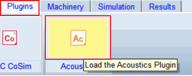
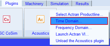
4. On the Plugins tab of the ribbon inside the Acoustics container, click the Actran logo to load the plugin:
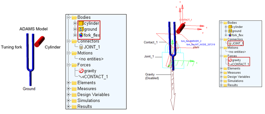
5. The model should now be open in the Adams View session. Familiarize yourself with it. It consists of a tuning fork flexible body, "fork_flex," and rigid body "cylinder" part that has an initial velocity in order to strike the tuning fork. The tuning fork is fixed to ground and there is a contact force between it and the cylinder. Gravity is disabled.
6. Generating Adams results:
■Simulate the Adams model:
a. Go to the Simulation tab
b. Click on the button Run a Scripted Simulation
c. Enter the Script Name ".tuning_fork.SIM_SCRIPT_dynamic_run"
d. Uncheck Update graphics display
e. Start the Simulation
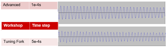
The simulation is performed with a time step  to
to 
to ■Verify the results loaded in the model browser.
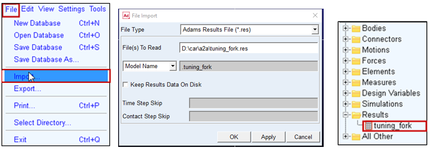
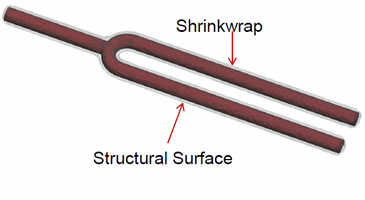
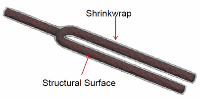
7. Modify Shrinkwrap: The acoustic mesh consists of: Shrinkwrap, Acoustic elements, Infinite elements. The shrinkwrap connects the structural mesh with the acoustic mesh. The acoustic mesh is directly connected to the shrinkwrap. The aim is to coarsen the shrinkwrap to reduce the number of elements while keeping the accuracy high enough. Use the "fork_shrinkwrap.bdf" file as the input file from working directory.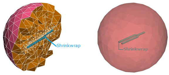
8. Edit Shrinkwrap file with ActranVI:
Note: | Actran license is required for this step. |
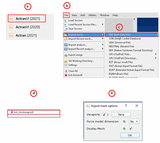
a. Open ActranVI (for example, on Windows) from the Start Menu under FFT - ActranVI [2021]
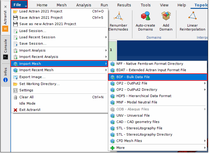
b. Go to the File tab and select Import mesh.
c. From the options available select BDF (Bulk Data File)
d. Browse and select the file fork_shrinkwrap.bdf.
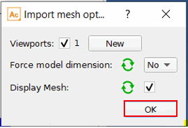
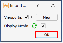
e. Import mesh options window will pop up, click OK
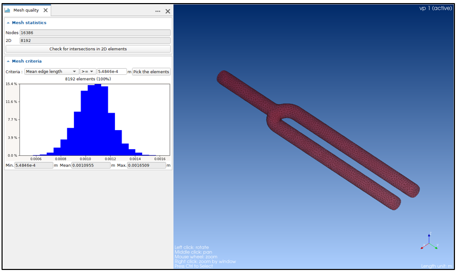
9. The Shrinkwrap Mesh will be displayed. The symbols on the left panel can be used to modify the view of the Shrinkwrap.
♦Blue points - to change the visibility of the element sets.
♦Cubes - to change the visibility of the grid
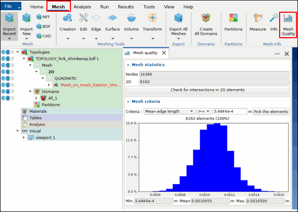
The Topology consists of a 2D mesh with Quadratic interpolation.
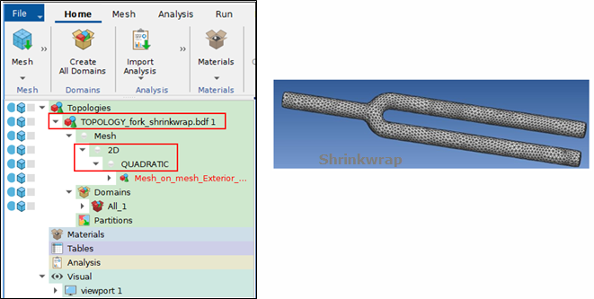
a. Select the 2D shrinkwrap mesh and Press Ctrl and left click on the mesh, the mesh will turn red in color.
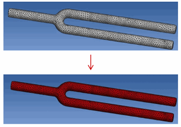
b. Go to the Mesh tab and then select Mesh quality tab. The mean size of the surface mesh is about 1e-3m, which is very fine to compute the sound propagation.
c. The mesh size can be coarsened. For a computation up to 1000Hz a mesh size of
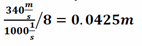
is sufficient if one creates 8 elements per wavelength for a frequency of 1000Hz (the speed of sound was assumed to be 340m/s)
d. The difference of the element size between fluid and structure should be kept to an acceptable ratio. Therefore, a 3mm mesh can be chosen.
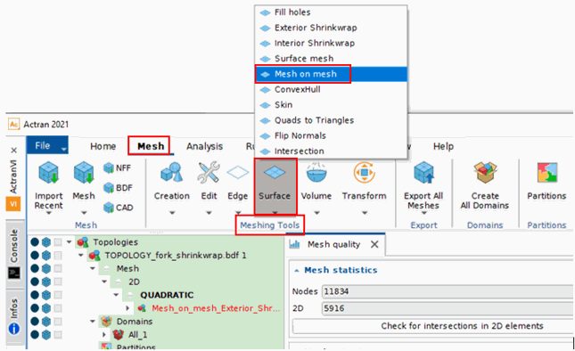
e. Go to Mesh tab and click on Meshing Tools -> Surface and select the Mesh on Mesh tool.
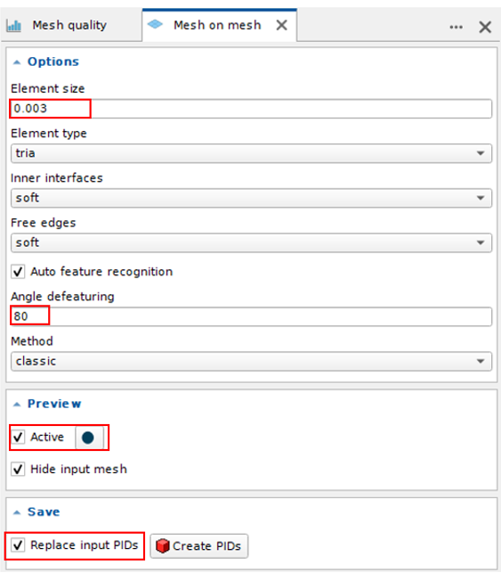
f. Set the parameters as follows:
♦Element size - 0.003m
♦Angle defeaturing - 80.0 °
♦Tick the preview- Active
♦Tick Replace Input PIDs
♦Click Create PIDs
The Shrinkwrap is now replaced by a coarser mesh.
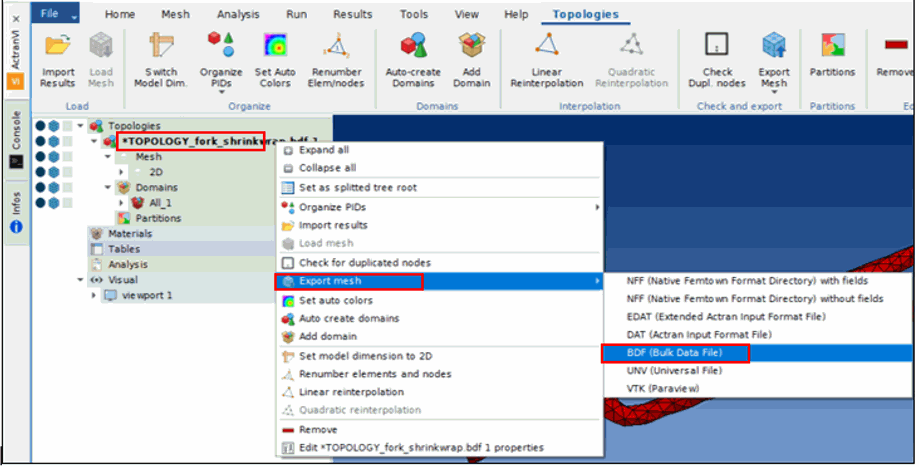
g. Export the mesh
♦In the left panel, right click on *TOPOLOGY_fork_shrinkwrap.bdf 1
♦Select Export Mesh and then Select BDF (Bulk Data File)
♦Keep the Output Format Selection as Short
♦Select file fork_shrinkwrap.bdf in the file browser dialog box, click on "Save" and say 'Yes' for replacing the file.
h. Two surfaces need to be connected, so that the vibration can propagate from the structure to the acoustic mesh. This is done with an interface connecting
♦the acoustic mesh (Shrinkwrap)
♦and the structural mesh (structural surface)
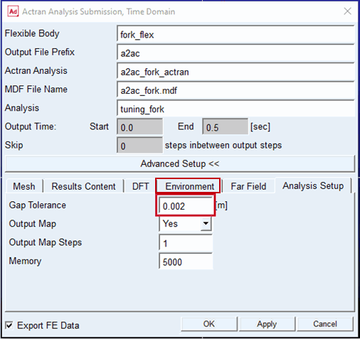
i. Within Actran a mapping algorithm is utilized to connect the structural and acoustic mesh. Within Adams Actran Analysis Submission, Time Domain dialog box, the gap tolerance is defined in the Advanced Setup under Analysis Setup. In order to optimize this value, the mapping can be checked within Actran VI.
10. Import the Structural Mesh
a. In the current session, go to File, click on Import mesh and select BDF (Bulk Data File)
b. Import the file fork_skin_mesh.bdf from the input files folder
c. Import mesh options window will pop up, Click OK.
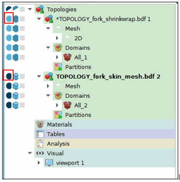
d. Both 2D meshes are now displayed.
e. 2D meshes are stored in 2 different topologies. To visualize both meshes at the same time, the first topology should be set to transparent and the second to opaque. This can be done by clicking on the small spheres next to the topologies. (In the left panel)
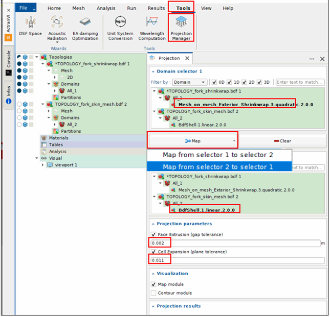
11. Mapping Control
a. Go to Tools and click on Projection Manager
b. Select the surface parameters as below:
c. Cell Expansion (Plane tolerance) - 0.011
d. Face Extrusion (Gap Tolerance) - 0.002m
e. Click on the  Button
Buttonf. Select Map from Selector 2 to Selector 1
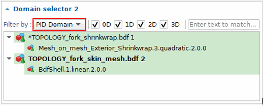
g. After selecting the Map the window will pop-up saying "Select domain first". Set the Domain to PID Domain.
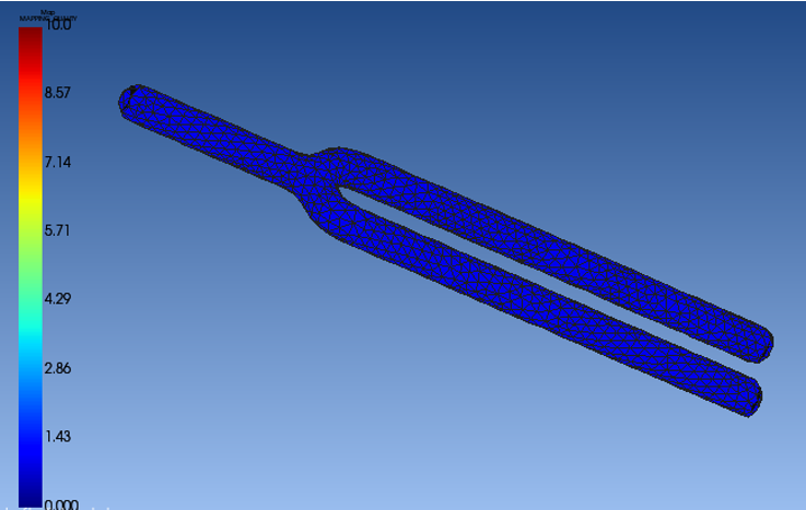
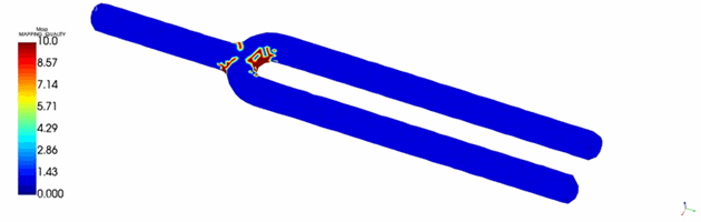
h. The mapping will be displayed.
♦Blue color indicates that all nodes have been found
♦Red color indicates the elements which are not connected
For a Gap Tolerance of 0.002 m, all nodes have been found and are connected.
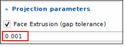
i. Redo the mapping with a Gap Tolerance of 0.001 m and Click on
In this case, a few areas of the shrinkwrap are red, indicating these areas are not coupled with the structure. Thus, Gap Tolerance of 0.002 should be used.
12. Create Actran Analysis
a. Go to the tab Plugins and click on the Acoustics plugin and select Time Domain.
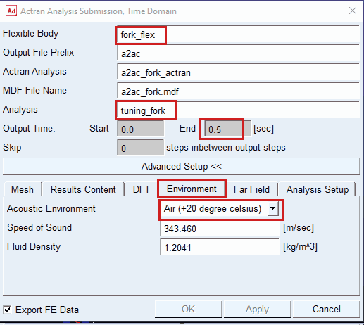
b. Double click to select the "fork_flex" as Flexible Body
c. Analysis - tuning_fork
d. Computational time (Output Time) End = 0.5 sec
e. Click on the Advanced Setup button and select Environment Tab.
Set Acoustic Environment = Air (+20 °C)
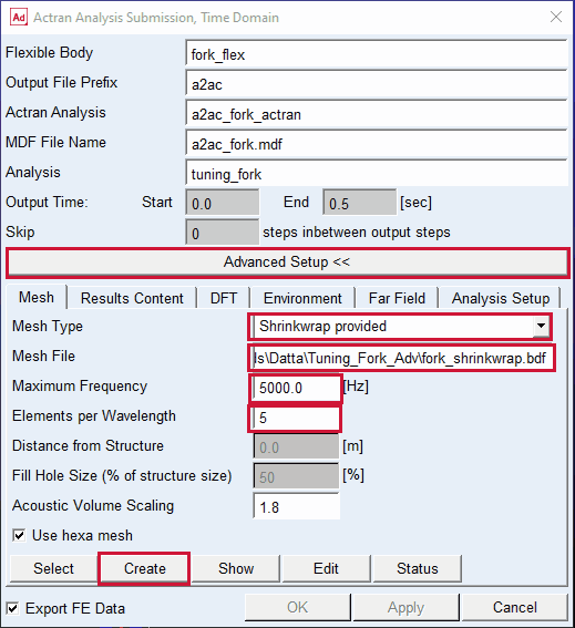
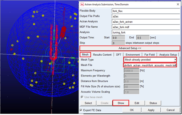
f. Click on the Mesh tab (under Advanced Setup) and set following parameters
♦Mesh Type - Shrinkwrap provided
♦Mesh File - fork_shrinkwrap.bdf (browse from working directory)
♦Maximum Frequency - 5000Hz
♦Elements per Wavelength - 5
Click on Create to create the acoustic mesh
g. Click on 'Show' Button to check the position of the microphone.
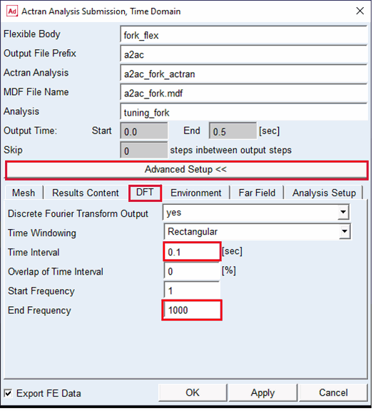
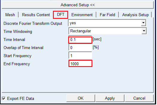
h. Go to the DFT tab and set the parameters as follows:
■Time interval - 0.1s
■End Frequency - 1000Hz
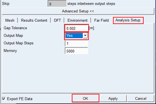
i. Go to the Analysis Setup tab and set following parameters.
■Gap tolerance should be set according to the mapping control test performed. So, set it to 0.002m.
■Output Map - yes
■Click on OK to generate the Actran analysis and the *.bat file to run the analysis.
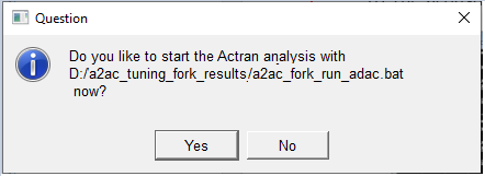
13. Choose Yes to start Actran analysis
■You can select No if you want to edit the parameter file (a2ac_fork_actran.par) and submit the analysis manually.
This will complete the computation.
14. Re-Launch Computation: Once the run in step 12 is complete, user can relaunch the computation by editing the batch file.
The analysis can now be run by the batch file in the working directory.
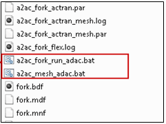
a. Go to the working directory where the files can be found
■The file a2ac_fork_run_adac.bat located in working directory/fork_actran_mesh folder can be used to run the Actran analysis
■The file a2ac_mesh_adac.bat located in working directory/a2ac_tuning_fork_results_* folders can be used to generate the acoustic mesh
b. Right click on the file a2ac_fork_run_adac.bat and open in text editor.
c. The file will be shown in the right panel.
■The lines which start with 'call' or 'copy' will be executed.
■'Echo' is used to add comments. The lines starting with the word 'echo' will not be executed.
■The Actran sequence consists of 3 steps:
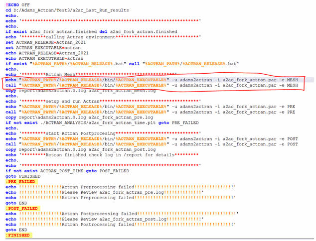
♦-e MESH to generate the mesh
♦-e PRE to generate the acoustic analysis and run the calculation
♦-e POST to do the post processing and sort the images
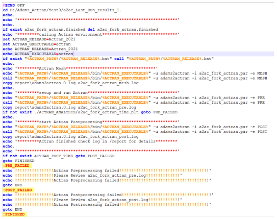
d. The acoustic mesh is already generated. Comment those lines with echo and Save the modifications
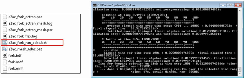
e. Run the analysis by double clicking on the a2ac_fork_run_adac.bat file.
15. Post Processing
a. The output map can be used to visualize different results over the entire fluid domain per time step, for example, the relative acoustic pressure or the fluid potential.
b. ActranVI can be used to display those results or to create an animation and save it as video file.
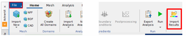
16. Import Output Map
a. Open ActranVI[2021]
b. Go to File -> Import mesh -> NFF - Native Femtown Format Directory. Select the folder a2ac_fork_map.nff from the file browser. (Note that the output map is in folder format)
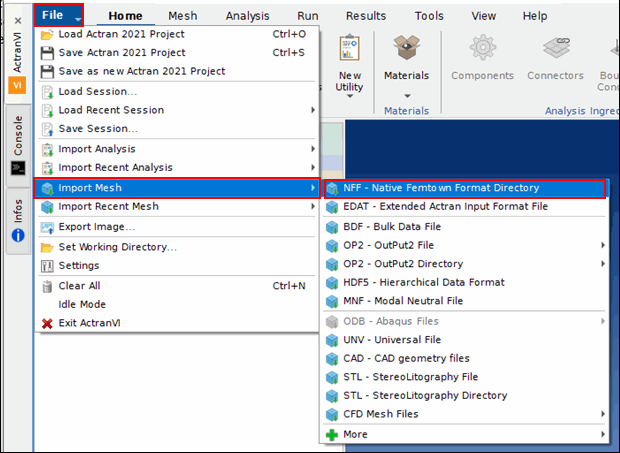
c. Click on OK
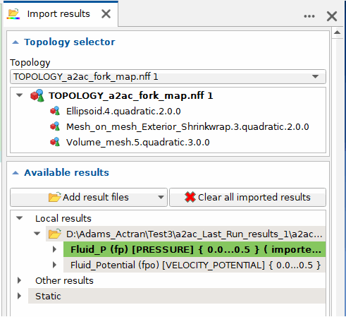
17. Visualize Output Map
a. Go to Import results
b. Double click on Fluid_P (Fluid Pressure)
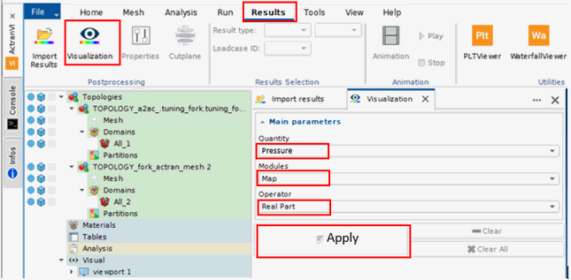
18. Go to Results menu and click on Visualization
Set the parameters as follows:
■Quantity - Pressure
■Modules - Map
■Operator - Real Part
Click on Apply
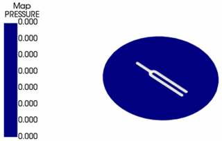
19. The Sound Pressure is displayed at t = 0.0s

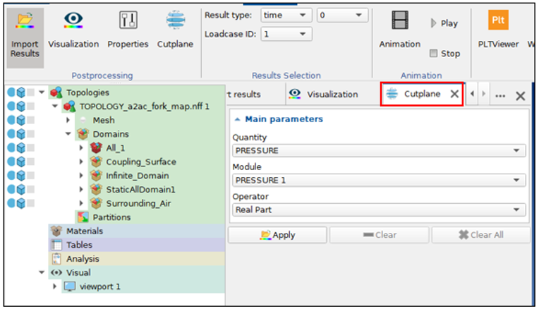
20. In Results menu, go to Cutplane and Click on Apply, the 3D domain is now cut by the defined plane.
21. In Results menu, go to Properties, select cutplane and select Z axis
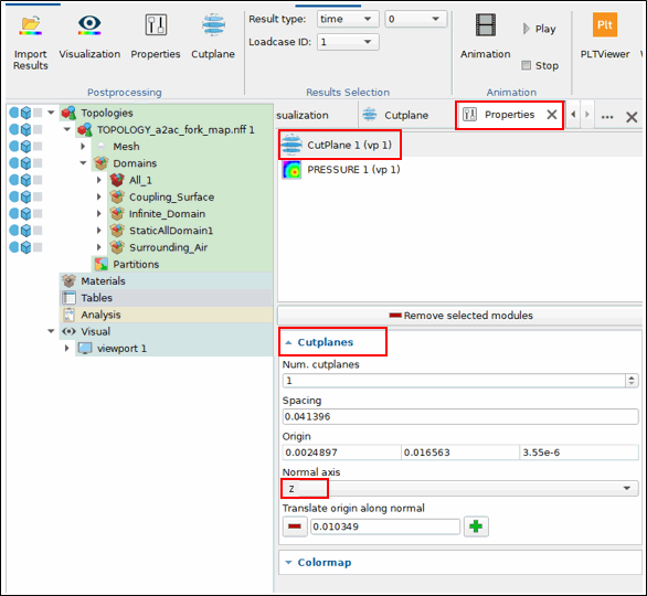
22. The tuning fork is cut in the z-axis
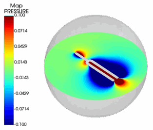
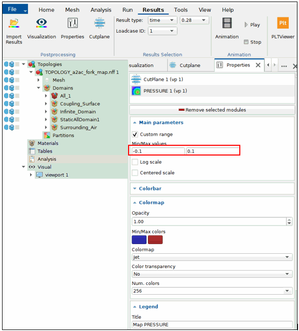
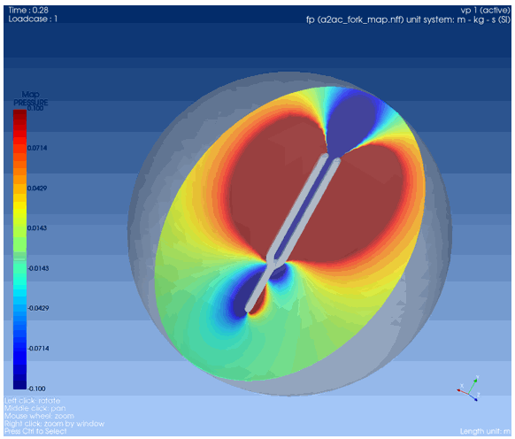
23. In Properties, Select Map pressure
a. Choose Min. Color to -0.1Pa (relative sound pressure)
b. Max. Color to 0.1Pa (relative sound pressure)
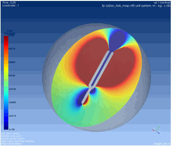
c. Time 0.28s
24. The sound pressure is visualized at 0.28s
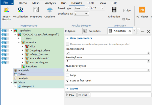
25. Start Animation
a. Click on Animation button located in Results menu, under Animation container
b. Choose Result Type: Time
c. Click on Play button
26. Generate MDF file: The MDF file is already available in the folder, here another possibility to generate the MDF file is shown
a. During the simulation of an Adams simulation with flexible bodies the modal participations of the flexible body are stored at each time step
b. Those can be visualized with Actran Waterfall Viewer (Actran Basic license necessary). The Output is done within the Durability plugin.
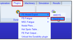
♦Go to the Plugins tab
♦Select the Durability Plugin
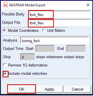
♦Select FE Modal Export and then select Nastran
♦Select the Flexible Body fork_flex
♦Output File fork_flex
♦Include modal velocities - yes
♦An mdf file with the name fork_flex.mdf is created
27. Load the MDF file in WaterfallViewer
Note: | Actran license is required for this step. |
Open the WaterfallViewer in the start menu under programs/FFT/Actran2021
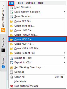
a. Go to File / Open MDF file
b. Import the file fork_flex.mdf
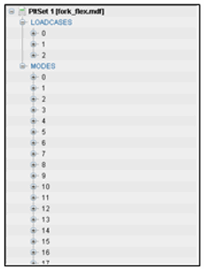
c. The file and its content is now displayed on the top left side
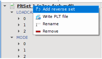
28. Visualize the Participation Factors
a. Right click on PLTSet and Add a reversed set
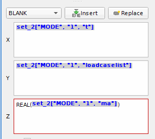
b. Expand Reversed PltSet and Mode 1. (Velocities) and right click on M_Amplitude and click on Plot REAL
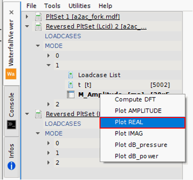
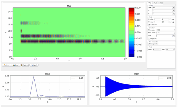
c. The fields are automatically filled and the modal participations are plotted
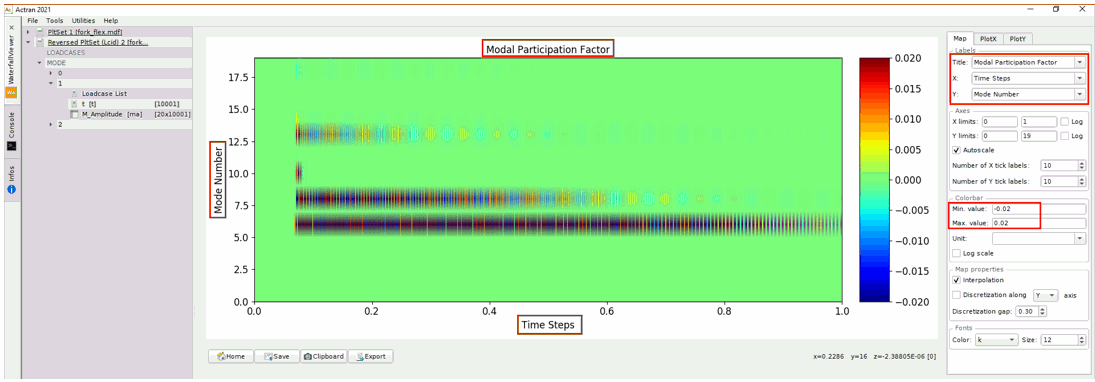
d. Modify Labels as follows:
♦X Label - Time Steps
♦Y Label - Mode Number
♦Title - Modal Participation Factor
Modify the Min and max values to -0.02 and 0.02
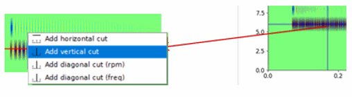
e. Plot Cut Views: By right clicking on the graph, cut lines can be added as shown in the image. Add a horizontal and a vertical cut to the plot.
29. Sound File: The finer time step of the simulation improves the sound quality of the results. Listen to the sound files generated in the
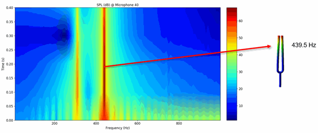
"A21-2_002_Adams_Acoustics_Time_Domain_Basic" and compare them with the files generated here. Finer time steps increase the sound quality. The frequency peak at 440Hz is captured with both time step sizes. Both simulations respect the Nyquist criterion for up to 1000Hz.
30. Remember that as part of the acoustics analysis a Fourier transform was computed with the settings.
■Time Interval - 0.1s
■Start Frequency - 1Hz
■End Frequency - 1000Hz
■Overlap of Time Interval - 0%
This generated the following output files in the working directory:
♦a2ac_fork_actran_micros_pa_40_DFT_dB.png
♦a2ac_fork_actran_micros_pa_40_DFT_Me
♦an_Pressure_Enevelope_dB.png
The images below show the DFT of five-time intervals (left side) and the envelope and mean values (right side) of both intervals
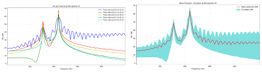
The frequency content of the time signals is found in the file "a2ac_fork_actran_micros_pa_40_DFT_waterfall_dB.png”
As in "A21-2_002_Adams_Acoustics_Time_Domain_Basic", The first mode of the tuning fork is driving the acoustic radiation