Steps to Run this Example
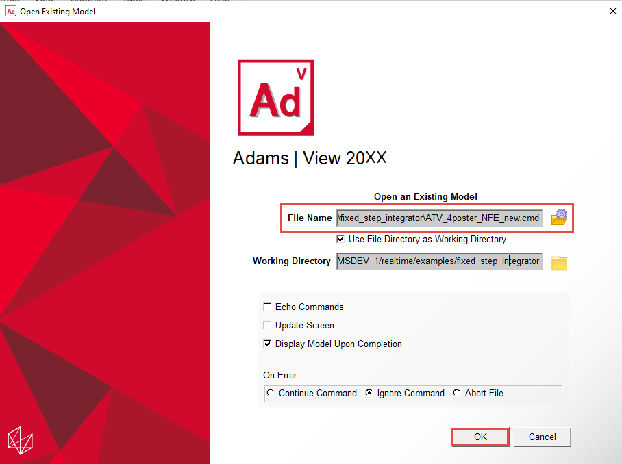
1. The files required for this tutorial can be found in the Adams installation at: \install_dir\realtime\examples\fixed_step_integrator\. Copy them to your working directory
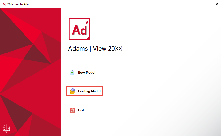
2. Start Adams View and choose to open an existing model
3. Choose to open the "ATV_4poster_NFE_new.cmd" file you copied from the Adams installation:
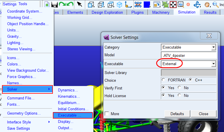
4. Go to Settings-Solver-Executable and set the "Executable" to "External" (this is not required to run the fixed step integration option, but allows us to see more output messages from Adams Solver)
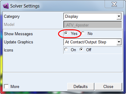
5. From the same dialog (Settings → Solver) pick Category = Display and for "Show Messages" select yes
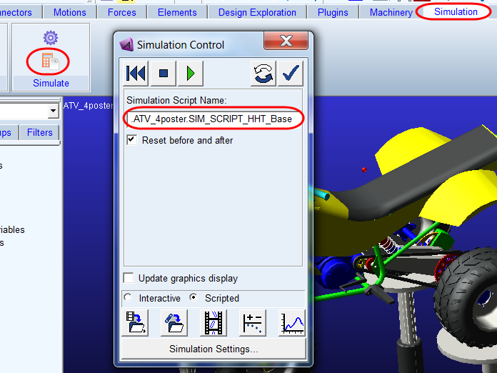
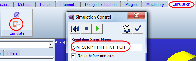
6. Click on Simulation tab and from the Simulate container click the Run a Scripted Simulation icon. Then choose the simulation script "SIM_SCRIPT_HHT_Base". This uses a traditional (variable time step) HHT integrator. Click the play button to run the simulation.
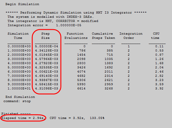
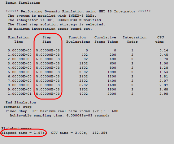
7. In the Information window notice that the step size changes and note the elapsed time (elapsed time will vary by machine).
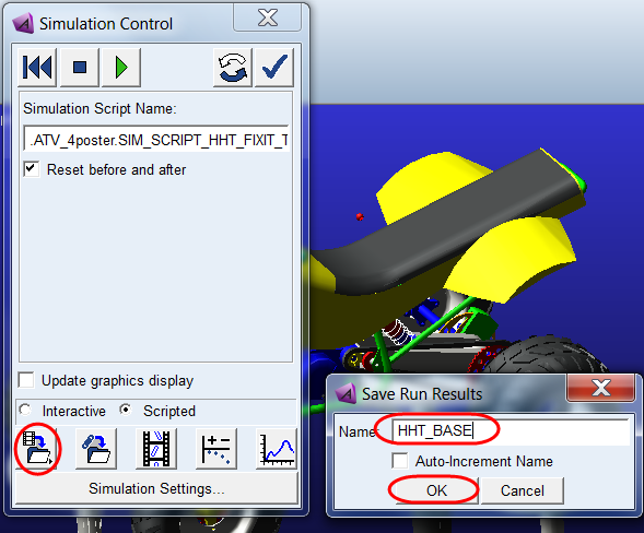
8. Save the analysis results as "HHT_BASE"
9. From the model browser click on the simulation script "SIM_SCRIPT_HHT_FIXIT_TIGHT" then right-click and select Info to display the details of the script.
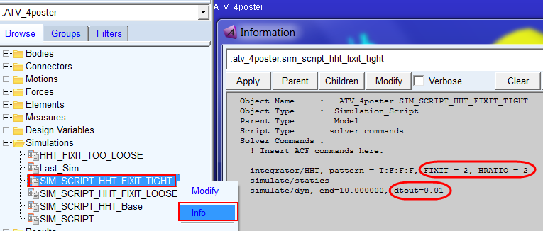
This script instructs Adams Solver to use the fixed step integration option with the HHT integrator (because FIXIT is specified on the integrator command). It instructs the solver to move ahead in time by fixed steps of 0.005s each. This is because…
♦dtout=0.01 means we want output steps at every 0.01s
♦HRATIO=2 means we want 2 solver steps within that 0.01s output step size; so, we have dtout/HRATIO = 0.01/2 = 0.005
♦FIXIT=2 means we want to the solver to take exactly 2 iterations per solver step then proceed (there is no regard for error tolerance when FIXIT is employed)
10. Now run a simulation using this script, "SIM_SCRIPT_HHT_FIXIT_TIGHT"
Notice this time we get a constant step size and note the elapsed time is smaller than the base run with the variable step integration:
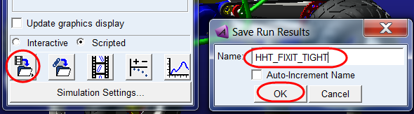
11. Save the results as "HHT_FIXIT_TIGHT"
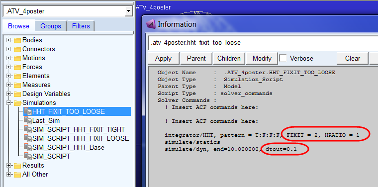
12. Now display Info for the simulation script SIM_SCRIPT_HHT_FIXIT_LOOSE
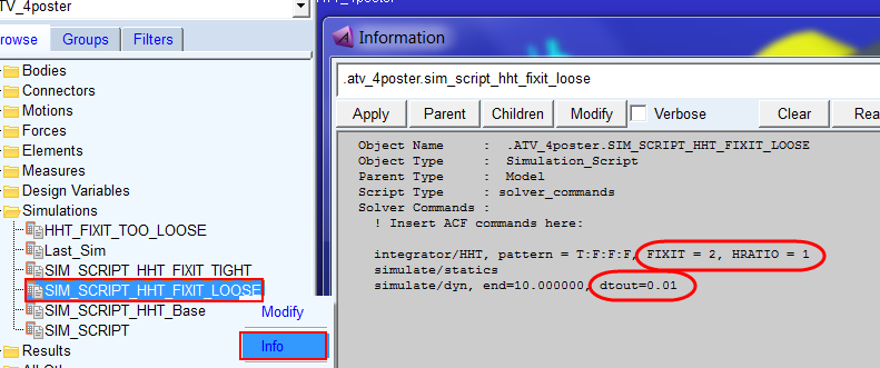
Here we still have FIXIT=2, but dtout/HRATIO = 0.01/1 = 0.01 (that is, larger solver step size than the tight script's settings)
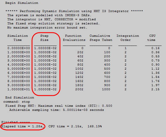
13. Run a simulation using this script, "SIM_SCRIPT_HHT_FIXIT_LOOSE"
Notice again a constant step size (this time at 0.01s) and, now, an even faster elapsed time:
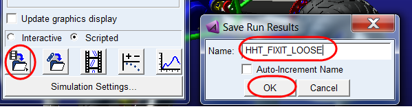
14. Save the results as "HHT_FIXIT_LOOSE"
15. Now display Info for the simulation script SIM_SCRIPT_HHT_FIXIT_TOO LOOSE
Here we still have FIXIT=2 but dtout/HRATIO = 0.1/1 = 0.1 (that is, larger solver step size than the loose script's settings)
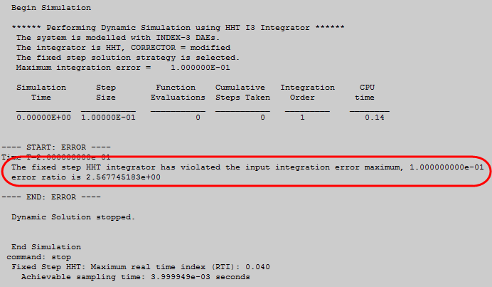
16. Run a simulation using this script, "HHT_FIXIT_TOO_LOOSE" This simulation fails pre-maturely with the error:
---- START: ERROR ----
STFINT:EUL_SINGULARITY.
Time=2.000000000E-01. Step=1.000000000E-01. The integrator has encountered a recurring Euler singularity which cannot be resolved and may be non-physical.
Suggested course of action :
1. Use the command debug/eprint to identify if there are any unconverged integrator time steps.
Note that too high corrector residuals/deltas may lead to non-physical Euler singularity.
2. Try changing dtout/hratio or fixit to avoid the unconverged integrator time steps.
3. Set MAXERR appropriately to stop the simulation in case of the unconverged steps (i.e. too high residuals/deltas in corrector iteration).
---- END: ERROR ---
The dtout/hratio determines the integration step size which is too large here. The corrector fails to converge in FIXIT number of iterations and eventually it leads to a repetitive Euler Singularity (Note that regular Euler Singularity is supported in the fixed step integrator).
Note: | Because of the high error experienced here, the same result (Euler Singularity at time 0.2) may not occur on all platforms in all Adams versions. Regardless, the point here is to illustrate the use of MAXERR to self-terminate an analysis; so, continue on below… |
This sort of singularity is more likely to occur when the error is very high. So, let's take the advice of item #3 in the error message and use the MAXERR argument to force the simulation to stop with such high error.
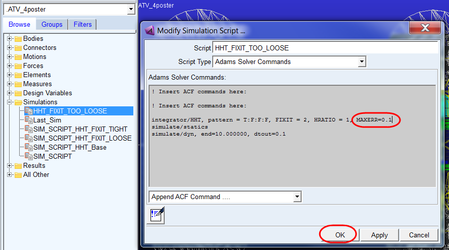
17. From the model browser open the "Simulations" folder and double click the simulation script "HHT_FIXIT_TOO_LOOSE" in order to modify it. Add "MAXERR=0.1" to the INTEGRATOR command as shown below. This will instruct Adams Solver to terminate the analysis as soon as the error goes above 0.1.
18. Now re-run a simulation using the script, "HHT_FIXIT_TOO_LOOSE". The simulation now terminates prior to encountering the Euler singularity:
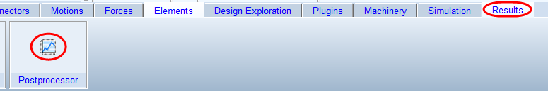
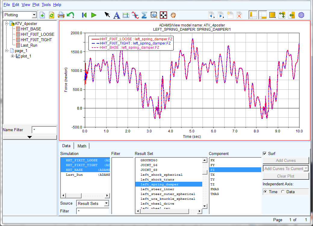
19. Go to Adams PostProcessor and compare the results for the force in one of the spring dampers.
20. Zoom in on the results near time = 0
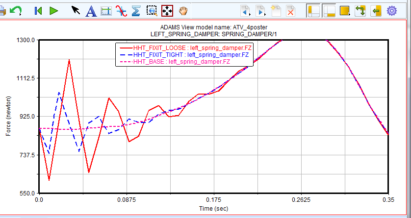
21. Compare different result channels and notice how accuracy changes with your dtout/hratio and fixit settings. In practice you will of course need to find the balance between speed and accuracy that is acceptable to you for your specific model and usage scanario.