Plotting Frequency Response
Next, you plot the magnitude and phase of the frequency response. Magnitude is plotted in decibels (dB) against a logarithmic (log) scale for frequency. Phase is plotted in degrees using linear scale against a log scale for frequency. This plot will help you understand how the vertical vibration from the rocket affects the solar panel response.
To plot frequency response magnitude:
1. Select the New Page tool  .
.
. 2. From the pull-down menu located below the File menu, select Plotting.
Adams PostProcessor switches to plotting mode.
3. Set Source to Frequency Response.
4. From the Vibration Analysis list, select vertical.
5. From the Input Channels list, select input_y.
6. From the Output Channels list, select p1_corner_y_acc.
7. Select Magnitude.
8. Select Add Curves.
9. From the Output Channels list, select ref_y_acc.
10. Select Add Curves.
Adams PostProcessor plots the frequency response magnitude.
To display a horizontal, two-page layout:
■Right-click the Page Layout tool  , and select the Horizontal, 2-page tool
  .
.
, and select the Horizontal, 2-page tool .■The viewport now contains the frequency response function plot and a blank plot.
To plot frequency response phase:
1. Select the blank plot.
2. Set Source to Frequency Response.
3. From the Vibration Analysis list, select vertical.
4. From the Input Channels list, select input_y.
5. From the Output Channels list, select p1_corner_y_acc.
6. Select Phase.
7. Select Add Curves.
8. From the Output Channels list, select ref_y_acc.
9. Select Add Curves.
Adams PostProcessor plots the frequency response phase.
From these plots you can determine the two primary modes that affect the vertical acceleration response. The first prominent mode is around 2.5 Hz. The second prominent mode is just above 10 Hz. These two modes contribute to an attenuation of accelerations about 4 Hz. This can be seen by comparing the input acceleration (ref_y_acc) directly with the output acceleration.
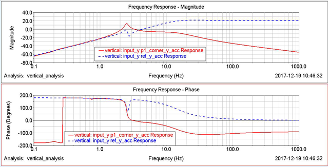
Figure 5 Frequency Response Plot