Adams Car Package > Adams Car > Reviewing Results > Plot Configuration Files

Plot Configuration Files

You can plot the results of an analysis using the standard functionality in Adams PostProcessor. To help you manage your plots, however, your template-based product provides plot configuration files that define a series of plots.

For information on Adams PostProcessor, see the Adams PostProcessor online help.

Learn more about plot configuration files:

■About Plot Configuration Files

■Creating Plots Using a Plot Configuration File

■Creating Plot Configuration Files

■Format of Plot Configuration Files

■Example Plot Configuration File

About Plot Configuration Files

Plot configuration files tell your template-based product:

■Which plots to create

■The layout of each page and the plots to be displayed on that page

■General settings and preferences, such as titles, labels, horizontal and vertical spacings, scaling, legend text and its attributes, axes positions and their attributes

■The mathematical expressions to be displayed for the plot axes

■The primary and secondary grid attributes for each plot

■The presentation of the plot, that is, whether it should show actual curves or the curve data in tabular format

■The text/images to be displayed for the header/footer of each page

■The date and analysis stamp related details

■The Note and Spec Line related details

The files now support multiple plots per page, and each plot can contain multiple axes. You can cross-plot multiple analyses of the same type using one plot configuration file.

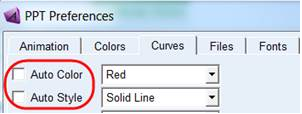
If you do not want Adams PostProcessor to auto-increment curve color and curve style (for example, because you want them assigned as you have specified in the plot configuration file), then you need to turn off automatic assignment of these attributes. From the Adams PostProcessor text menu select Edit → Preferences and go to the Curves tab. From there un-check "Auto Color" and "Auto Style" as shown below:

Plot configuration files are TeimOrbit files and are stored in your database in the plot_configs.tbl directory. See TeimOrbit File Format.

You can access the plot configuration file functionality in Adams PostProcessor. Learn about creating a plot configuration file through the interface. Learn about using plot configuration files.

Note:

To modify plots and curves, you can use the command statement in each block to invoke macros, which must contain the modification commands. The macros must be contained in your current binary file, which can be either private or site.

Creating Plots Using a Plot Configuration File

After you've run an analysis, you can view the series of plots defined in a plot configuration file. If your plot configuration file contains customization command keywords and it has created the plots and curves, you can have your template-based product invoke the macro that contains a command keyword in its user-entered command.

The plot configuration file specifies a subtitle for your plots. In addition, in the File Import dialog box you can:

■Add a title to all the plots.

■Plot results of multiple analyses on one plot using the Cross Plotting option.

■Change the look of your plot, such as fonts and size, using the Execute Custom Macros option. To use this option, you must have a macro that defines the commands to be executed.

To view the plots defined in a plot configuration file:

1. From the Review menu, select Postprocessing Window or press F8.

2. From the File menu, point to Import, and then select Plot Config File.

The File Import dialog box appears.

3. In the Analyses text box, enter the analysis or analyses from which you want to view results.

4. In the Plot Configuration File text box, enter the name of the plot configuration file defining the plots that you want to view.

5. In the Plot Title text box, enter the title to appear at the top of the plots.

6. Select Cross Plotting to plot analysis data on existing plots containing data from other analyses.

If you selected multiple analyses in the Analyses text box, your template-based product automatically plots the data from the different analyses on the same plots.

7. If you have customization command keywords in the plot configuration file you selected in Step 4, then select Execute Custom Macro.

Your template-based product invokes the macro which executes any commands that customize the plots.

8. Select OK.

Creating Plot Configuration Files

You can create a plot configuration file containing all of the pages currently in Adams PostProcessor or only a selected set of pages. Your template-based product stores the configuration files in the plot_config table of your default writable database. Learn about Setting the Writable Database.

To create a plot configuration file:

1. From the Review menu, select Postprocessing Window or press F8.

2. Create and configure plots as desired, including specifying labels and spacing. For example, you can create a set of plots and add subtitles to all of them that describe the type of analysis with which the plots are associated.

3. Customize plots to suit your requirements. For example, you can assemble multiple plots on the same page by changing the page layout. To change the page layout, from the View menu, point to Page and then select Page Layouts. This will display the Page Layouts dialog box. Select the desired layout.

4. Change the appearance of the plot if you would like to see the curve data in tabular format. To change the plot to tabular format, click on the associated plot and check the checkbox for Table shown at the bottom left. This setting is saved in the plot configuration file and the plot will be seen in the tabular format when this file is imported in future.

5. Add Notes or Spec Lines to the plot. To do this, from the Plot menu, select Create Note or Create Spec Line. On the respective dialog box, specify the data for the Note or Spec Line.

6. Specify the text or images for the header/footer of the pages. To do this, select the required page and point to Header or Footer tabs shown at the bottom left area. Each of these tabs have subtabs like Left, Center and Right. You can specify the text/image for them. To specify image for the header/footer. Select any of these subtabs and set the Source to Image. This displays the Image field below the Source field. You can double-click in this field and browse to the required image for the header/footer in any location - Left, Center or Right.

7. Customize the appearance of legend, axes, curve, date and analysis stamp as per your requirement. To do this, you can select these entities from the plot or select their entries from the tree view. Depending on the type of entity, various options/tabs are available in the lower left corner to modify associated properties.

8. From the File menu, point to Export, and then select Plot Configuration File.

The Save Plot Configuration File dialog box appears.

9. In the Configuration File Name text box, enter the name for the plot configuration.

10. If you want to include all pages currently in the Plotting window, select All Pages.

11. If you did not select All Pages, in the Page Name(s) text box, enter the names of the pages that you want to include in the plot configuration file.

12. In the Plots and Curves text boxes, enter command keyword to invoke the macro that customizes the plots and curves.

Your template-based product saves the command keyword with your plotting configuration file. After it creates the plots and curves, your plotting configuration file invokes the macro which contains the commands.

13. Select OK.

14. This exports the plot configuration file with the specified name. If you specify images for the header/footer of any page, these image files are copied to the location where the plot configuration file is saved.

Format of Plot Configuration Files

Plot configuration files consist of three data blocks:

■Page Data Block

■Plot Data Block

■Plot-Curve Data Block

Page Data Block

The Page data block has the following structure:

PAGE_LAYOUT

NUMBER_OF_PLOTS

PAGE_NAME

HEADER/FOOTER

Header/Footer data: This section will be present only if you have specified text/image for any section (Left, Center or Right) of Header or Footer. The entries are present only for those sections for which the text/image is specified.

Plot Data Block

The plot data block has the following structure:

INDEX

NAME

TIME_LOWER_LIMIT

TIME_UPPER_LIMIT

LEGEND (subblock)

PLOT_BORDER (subblock)

PRIMARY_GRID (subblock)

SECONDARY_GRID (subblock)

LEGEND_BORDER (subblock)

GRAPH_AREA (subblock)

SPEC_LINE (subblock)

NOTES (subblock)

PLOT_AXES_FORMAT (subblock)

PLOT_AXES_LABELS (subblock)

PLOT_AXES_TICS (subblock)

PLOT_AXES_NUMBERS (subblock)

CURVE_ATTRIBUTE_ORDER

COMMAND

CURVE_ATTRIBUTE_ORDER:This section will be present in plt file, if a plot contains multiple curves representing the exact same quantity and using the exact same expression then, for those curves, only one curve is saved to the .plt file, and the order in which curve attributes are applied to curves is stored per plot.

command_keyword

After your template-based product creates each plot, it executes the following commands if you defined a command keyword:

acar custom_plots <command_keyword> & plot_name=<plot_name>

The command acar custom_plots <command_keyword> must already be created in the current session, either interactively or already present in the acar.bin, file.

Plot-Curve Data Block

The plot-curve data block has the following structure:

NAME

PLOT

VERTICAL_AXIS

HORIZONTAL_AXIS

HORIZONTAL_EXPRESSION

HORIZONTAL_COMPONENT

VERTICAL_EXPRESSION

VERTICAL_COMPONENT

Y_UNITS

X_UNITS

LEGEND_TEXT

COLOR

red, blue, yellow, magenta, cyan, black, white, skyblue,

midnight_blue, blue_gray,dark_gray, silver, peach, maize

STYLE

solid, dash, dotdash, dot

SYMBOL

none, x, o, plus, star, at

LINE_WEIGHT

Real value from 1-4

COMMAND

command_keyword

HOTPOINT

INCREMENT_SYMBOL

After your template-based product creates each curve, it executes the following commands if you defined a command keyword:

acar custom_plots <command_keyword> &

analysis=<analysis> &

plot_name=<plot_name> &

vertical_data=<y> &

horizontal_data=<x> &

curve_name=<curve_name>

The command acar custom_plots <command_keyword> must already be created in the current session, either interactively or already present in the acar.bin, file.

Example Plot Configuration File

The following is an example of an Adams Car plot configuration file:

$--------------------------------------------------------------MDI_HEADER

[MDI_HEADER]

FILE_TYPE = 'plt'

FILE_VERSION = 2.0

FILE_FORMAT = 'ASCII'

$-----------------------------------------------------------------------PAGE

[PAGE]

PAGE_LAYOUT = 11.0

NUMBER_OF_PLOTS = 1.0

PAGE_NAME = 'my_page'

HEADER_LEFT_LINES = 1.0

HEADER_LEFT_LINE_0_TEXT = 'Header Left'

HEADER_LEFT_TEXT_FONT_SIZE = 7.0

HEADER_LEFT_COLOR = 788529153.0

FOOTER_RIGHT_LINES = 1.0

FOOTER_RIGHT_LINE_0_TEXT = 'Footer Right'

FOOTER_RIGHT_TEXT_FONT_SIZE = 15.0

FOOTER_RIGHT_COLOR = 788529232.0

$-----------------------------------------------------------------------PLOT

[PLOT]

INDEX = 0.0

NAME = 'my_plot'

TIME_LOWER_LIMIT = 0.0

TIME_UPPER_LIMIT = 0.0

(LEGEND)

{placement location fill grow_left grow_down font}

'bottom right' 156.8,10.6 1 TRUE FALSE 7

(PLOT_BORDER)

{color line_style line_weight}

'BLACK' 'solid' 1.0

(PRIMARY_GRID)

{color line_style line_weight}

'SILVER' 'solid' 0.5

(SECONDARY_GRID)

{color line_style line_weight}

'SILVER' 'solid' 0.5

(LEGEND_BORDER)

{color line_style line_weight} '

BLACK' 'solid' 1.0

(GRAPH_AREA)

{minX minY maxX maxY auto_graph_area}

8.5989 8.1158 159.3194 88.3882 yes

(SPEC_LINE)

{name color style location thickness}

'new_spec_line' 'Coral' 'dotdash' 10.0,10.0 1.0

(NOTES)