Theoretical background
This section presents a technical overview of the Adams Co-Simulation Interface (ACSI) implementation details. Granted that FMI for Co-simulation [5] is becoming increasingly popular, this document uses some FMI terminology to clarify some concepts.
Given that MSC is proprietor of both Adams and Marc computer codes, a decision was made to implement a custom co-simulation interface making use of the intimate knowledge of both codes resulting in an efficient co-simulation implementation. Moreover, the ACSI has been coded to support future enhancements.
The ACSI has the following specifications:
Communication architecture
The Glue code (also known as, primary code) implements a simple control algorithm allowing a variable asynchronous communication of the Adams and other codes (also known as, secondary codes) at each integration step. There are no restrictions imposed on the size of the time steps taken by both codes. The sole management is done to keep Adams running first and the other codes running last. The Glue code allows the other codes to go slightly ahead of Adams in some cases. All secondary codes simulate using their best settings. All secondary codes exchange data with the primary code at the end of every successful integration time step. In principle, all codes may have different integration steps.
This architecture does not require setting a communication interval like in some other co-simulation standards. During dynamic co-simulation, the communication with the Glue code is constant at the end of every integration step. This means the communication is more frequent if the co-simulation solution is difficult to compute. Similarly, the communication with the Glue code will be less frequent when the codes are taking larger step sizes. In a few words, there is no need to setup a communication interval.
Co-simulation setup
The Glue code controls the starting up and shutdown of all secondary codes. Users need to follow the prompts to launch the other codes. Starting with version ACSI 2016, the Glue code may launch the other processes automatically if they are running on the same host.
The topology (also known as graph G in FMI terminology) is defined using a simple configuration script. Adams, Marc and EDEM models need not to be exported into some other formats; instead users need to instrument the models following simple rules. Models can be modified quickly and a new co-simulation can be started immediately.
Interpolation/extrapolation algorithms
Core to all co-simulation codes there is a set of supported interpolation and extrapolation algorithms. The Glue code supports different interpolation/extrapolation algorithms for forces and displacements. The settings are global, future enhancements will allow users to set the algorithms on a model basis. The ACSI supports the following algorithms:
1. Quadratic
This option uses the past history of a signal (force or displacement) to exactly fit a quadratic curve through the last three available points in the history of the signal. The Glue code keeps a history of all transmitted data from all the secondary codes. To use this option set interpolate_order_u=2 and/or interpolate_order_f=2 in the configuration script.
2. Linear
This option uses a linear fit using a weighted slope s=s1*w + s2*(1-w) where s1 is the slope of the latest data time interval and s2 is the slope of the previous step. The weight w is provided by the user. For example, to use this option for displacements set interpolate_order_u=1 and say linear_weight_u=0.788 in the configuration script. Option linear_weight_u sets the weight w above. Similar options exist to set the interpolation/extrapolation for forces (see interpolate_order_f and linear_weight_f).
3. Constant last
This option uses the latest value in the history of the signal. To use this option set interpolation_order_u=0 and/or interpolation_order_f=0 in the configuration script.
4. Linear least squares
This option uses a least square linear fit of the last three values in the history of a signal. To use this option set interpolation_order_u=-1 and/or interpolation_order_f=-1 in the configuration script.
5. Constant average
This option uses the average of the last three values. This option is equivalent to using a constant least square fit on the data. To use this option set interpolation_order_u=-2 and/or interpolation_order_f=-2 in the configuration script.
Notes: | ■The above algorithms are supported for the interpolation/extrapolation of forces and translational displacements only. For rotational displacements, a SLERP algorithm is used to interpolate rotational displacements [6]. ■At start up, when the history of a signal does not have enough points for the selected interpolation algorithm, a simpler method is used. For example, a constant or linear interpolation is used. |
Main co-simulation algorithm - Force extrapolation case
When co-simulating with Marc versions earlier than 2015.0 or when co-simulating with EDEM, a simple force extrapolation algorithm is used. Starting ACSI 2015.0 Marc shares tangent stiffness information with the primary code and a different algorithm is used for that case. This section describes the simple algorithm when no stiffness information is shared. See next section for the case when Marc shares its tangent stiffness information.
For clarity, this section assumes a co-simulation with Marc only (the case of multiple Marc models and an EDEM model is similar). The main co-simulation algorithm belongs to the set of common co-simulation algorithms where Adams "goes first" using predicted forcing values from Marc. Later on, computed displacements by Adams are enforced in Marc using interpolated values.
Assume both Adams and Marc are at simulation time t1 and both are ready to move ahead in time and both are going to take the same integration step h. Figure 3 (a) and (b) show plots of the current force values (fc and fp) and displacement (u) values up to time t1 at one interaction point.
Figure 3 (a) shows the status of the Adams computation at time t1. Curve u is the computed displacement done by Adams while fp is the predicted force used by Adams. We have to stress the point that fp is not the force computed by Marc but values predicted by the Glue code using the computed values fc by Marc. More details follow.
Figure 3 (b) shows the status of the Marc computation at time t1. Curve u is the enforced displacement imposed by Adams; this curve matches the curve in Figure 3 (a). Curve fc is the computed force by Marc at the interaction point up to time t1. Notice point P stands for the predicted value of the force at time t1+h. This prediction is done by the Glue code (the Glue code keeps a history of all the force values from Marc.) The predicted value P will be used by Adams when starting to move ahead first. Notice the predicted value is obtained by extrapolation of the computed values by Marc (dotted line in Figure 3 (b)).
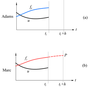
Figure 3 Adams and Marc at time t1 ready to move ahead in time.
Figure 4 (a) and (b) show the status of the co-simulation after both codes already took their respective simulation steps advancing in time. First, Adams advances its simulation using the extrapolated value P for the force at the interaction point (see Figure 4 (a).) Notice the value of P in the plot for fp. Next, Marc takes its simulation step using interpolated data u from Adams and computes the force C at the interaction point. The difference between the predicted value P and the computed value C is a measure of the error in the co-simulation.
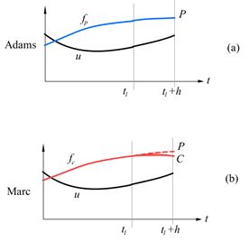
Figure 4 Adams and Marc after moving ahead one step.
In general, both fp and fc can be plotted by extracting the data from the Marc and Adams results sets.
Main co-simulation algorithm - Tangent stiffness case
Starting Marc version earlier 2015.0 a new co-simulation algorithm is used. Instead of using extrapolated force values from Marc, the Adams models uses the current extrapolated value of the force fp (see Figure 3) at the start of the time step plus a force equal to the tangent stiffness of Marc times the incremental displacements. In matrix form, for the case of single interaction, Adams applies the following force {fp} at the interaction point:
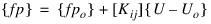
Here fpo is the extrapolated value of the computed Marc forces at the start of the Adams time step. The tangent stiffness matrix [Kij] is passed from Marc to Adams. Array Uo corresponds to the displacements at the interaction point at the start of the time step, and array {U} stands for the displacements at the interaction point.
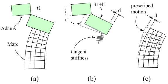
Figure 5 Using the tangent stiffness
The co-simulation algorithm doesn't define a fixed communication interval. Both codes run at their own settings. However, without loss of generality we assume both Adams and Marc models are at the same time t1 as shown in Figure 5 (a). Figure 5 (b) shows the Adams model taking a single time step h; notice that instead of using extrapolated forces during the whole time step, Adams uses the equation above that includes the tangent stiffness provided by Marc and a single extrapolated value at the beginning of the time step. Figure 5 (c) shows the Marc model simulating with the prescribed motion "d" imposed by Adams. (Here "d" stands for 3 displacements and 3 rotations.)
The value of the force computed by Adams at the end of the Adams time step is referred as P in the previous section. Notice P depends on the value of fpo provided by Marc. After Marc takes its time step (Figure 5 (c)), Marc computes the forces C. See Section Error control on how the ACSI monitors the error between these two forces.
Main co-simulation algorithm - Limitations
While the implemented algorithm provides good results, there are situations in which it is convenient to explicitly diminish the time step size in Adams. Most of the time 99% of the total simulation's wall time will be spent by the FEA codes, hence forcing Adams to take smaller time steps does not contribute significantly to the total simulation time. The typical problem in which it is necessary to diminish Adams time steps is the case of impact or sudden changes in the stiffness of the Marc model. To illustrate this issue, take for example the case of an imminent impact as shown in Figure 6.
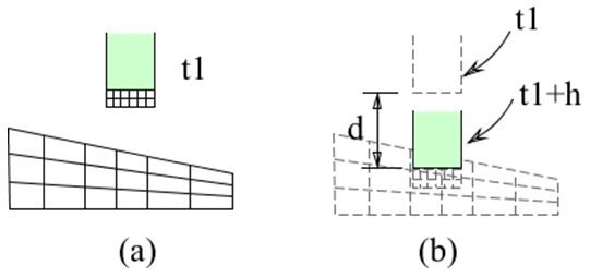
Figure 6 Impact co-simulation
Figure 6 (a) shows an Adams model (in green) moving on a free fall. The Marc model consists of two domains with a contact definition between them. If Adams is free to take a time step "h", the resulting displacement "d" shown in Figure 6 (b) will provide wrong results because the Adams will take the step using a negligible stiffness obtained at the beginning of the time step. A workaround consists of diminishing the time step so the imposed displacements "d" are small during the beginning of the impact. That way Adams will promptly "detect" the change of stiffness and the resulting co-simulation will be more accurate.
Notice this limitation is a consequence of the simplicity of the overall co-simulation algorithm regarding error correction. In fact, the ACSI does not reject the simulation steps taken by all codes if the computed error is beyond the prescribed errors. Future implementations of the ACSI will not suffer from this limitation.
Error control
Two conditions are constantly monitored for all components of forces and moments at all interaction points. When the absolute value difference between P and C (see previous sections) is bigger than an absolute error ea and the relative difference is bigger than a relative error er then a warning message is printed; nevertheless, the co-simulation does not stop. Both ea and er can be set by using the options force_absolute_error and/or force_relative_error in the configuration script. If both P and C are zero, the relative comparison is skipped.
The error condition (when P is not zero) is:
if( |P-C|>ea and |(P-C)/P|>er )
{
print warning message;
}
The warning message includes the interaction name (read from the configuration script) and the force/moment component name (for example, Fy). The error checking is performed at the end of every Adams simulation step taken.