Co-Simulation and Interpolation/Extrapolation
For co-simulation mode, the variables are not continuously in-sync with each other, as in Function Evaluation mode, since the variables passed between Adams and MATLAB/Simulink or Easy5 are sampled. Optionally, you can choose to interpolate/extrapolate these variables in between the sample times. The following is a brief description of how Adams Controls co-simulation interpolation/extrapolation works.
During co-simulation, if either Simulink or Easy5 is driving the analysis (that is, "leading the co-simulation"), single communication interval (delta) step consists of the following:
1. Easy5 or MATLAB/Simulink integrates from time = t - 1 to t to compute inputs for Adams Controls at time = t.
2. Easy5 or MATLAB/Simulink then requests outputs from Adams Controls at time = t.
3. Adams Controls integrates its equations until from t - 1 to t to provide outputs to Easy5 or MATLAB/Simulink.
4. Easy5 or MATLAB/Simulink takes the Adams outputs at time = t to complete the cycle and move on to integrate from t to t + 1.
During these four stages, in step 1, the inputs to Adams Controls can be interpolated or held constant, while in step 3, the outputs from Adams Controls can be extrapolated or held constant.
Interpolation/Extrapolation Options
Step 1 - Options for Adams Controls Plant Inputs
The following describe what happens to the Adams Plant inputs (that is, outputs from Easy5 or MATLAB/Simulink) when Simulink or Easy5 leads the co-simulation.
■If the Plant Input interpolation order is set to zero:
Adams Controls holds the Easy5/Simulink inputs, U, as constant values. In other words, apply a zero-order hold to the Plant Input values of Easy5 coming into Adams. For example, specify that the sample times occur at time = 0, 1, 2... If the current sample time is time = 2, and the last communication interval is time = 1, the Plant Inputs are sampled at time = 2, and held constant while Adams integrates from the last time (t1) to the current time (t2) to provide the Plant Outputs to Easy5.
■If the Plant Input interpolation order is set to one:
Adams Controls uses linear interpolation between the current and past values from Easy5 or MATLAB/Simulink. For example, if the current sample time is time= 2 (t2), and the last sample time is time = 1 (t2), the Plant Inputs are sampled by Adams Controls at time = 2, and linearly interpolated from t1 (saved from the previous communication time) to t2, as shown below while Adams integrates from the last time (t1) to the current time (t2) to provide the Plant Outputs to Easy5.
interpolation: Plant Inputs, U (1 → 2) = U1 + (U2 - U1) / communication_interval * (current_simulation_time - t1)
Step 3 - Options for Adams Controls Plant Outputs
The following describes what happens to the Adams Plant outputs (that is, inputs to Easy5 or MATLAB/Simulink)
■If the Plant Output extrapolation order is set to zero:
Easy5 or MATLAB/Simulink assumes that the Adams outputs (Y) are constant values. In other words, apply a zero-order hold to the Plant Output values of Adams coming into Easy5 or MATLAB/Simulink. For example, if the last sample time was time = 1, and the current sample time is time = 2, then Easy5 samples the Adams Plant Outputs at time = 1, and holds them constant while Easy5 integrates from the last time (t1) up to the current time (t2) to provide the Plant Inputs to Adams.
■If the Plant Output extrapolation order is set to one:
Easy5 or MATLAB/Simulink uses linear extrapolation beyond the past two values from Adams. For example, if the last sample time was time = 1, and the current sample time is time = 2, then Easy5 uses the saved samples of the Adams Plant Outputs at time = 1 and time = 0, and linearly extrapolates, as shown below while Easy5 integrates from the last time (t1) up to the current time (t2) to provide the Plant Inputs to Adams.
extrapolation: Plant Outputs, Y (1 → 2) = Y1 + (Y1 - Y0) / communication_interval * (current_simulation_time - t1)
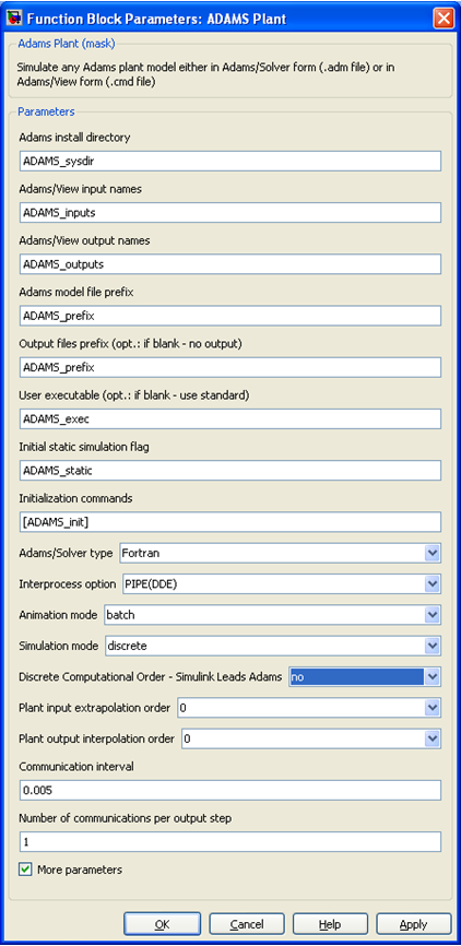
Only in Simulink, optionally, you can choose Adams to lead the co-simulation, which may be used to break an algebraic loop with the Adams Controls S-Function. In this case, the interpolation and extrapolation methods are exactly the same, but are reversed for the plant inputs and outputs (that is, the Plant Inputs are extrapolated and the Plant Outputs are interpolated). This setting can be seen highlighted below:
Example: Antenna Model
The following shows the antenna example found in the Getting Started Using Adams Controls for setting interpolation/extrapolation in Co-simulation vs. Function Evaluation. This example shows the effect of interpolation and extrapolation on the accuracy of the result, and also shows the effect of the communication interval on extrapolation. Here, Simulink leads the co-simulation.
The first plots show the antenna model output azimuth position for Function Evaluation (red curve) vs. co-simulation:
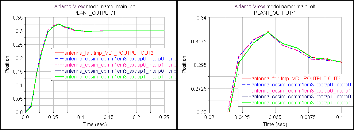
The communication interval is set to 1 millisecond, and the results for all interpolation settings are very close to the result for Function Evaluation. However, upon closer inspection, the plot on the right show that for linear extrapolation ("extrap1"), the co-simulation results (shown in the green line) are very close to the results for Function Evaluation. The results for extrapolation off are similar (red and blue striped line), but a little bit different than Function Evaluation. This can also be seen in the next plot of the input torque to Adams:
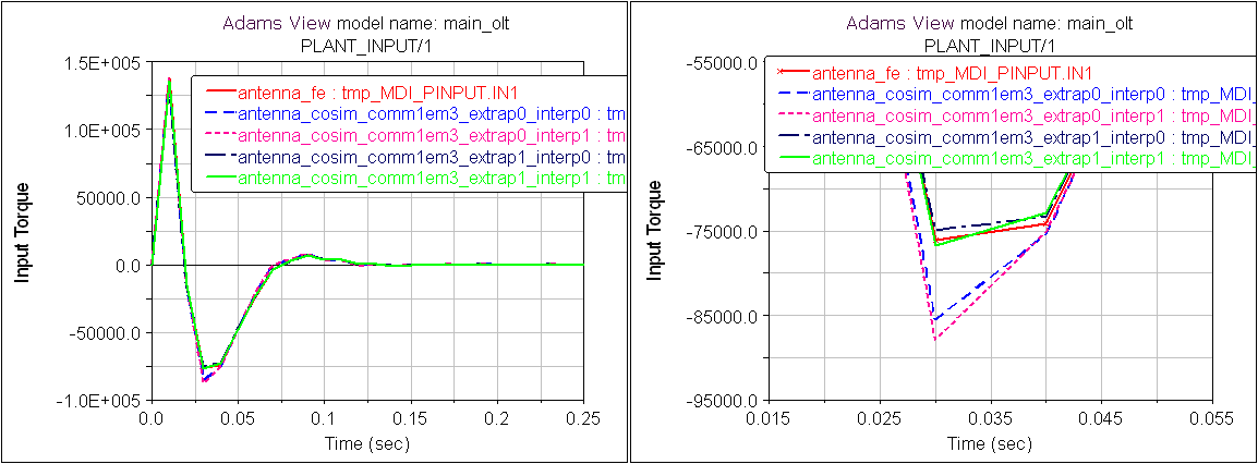
The plot to the right is a close-up of the bottom of the plot on the right. You can see that the red line for Function Evaluation is more closely matched by the plots that use extrapolation ("extrap1").
Now, for comparison, look at this same example where the communication interval has been changed from 1 ms to 5 ms. In this case, the linear extrapolation is not as accurate as for 1 ms, and the results without extrapolation appear to be closer to the Function Evaluation case.
Plot of azimuth position: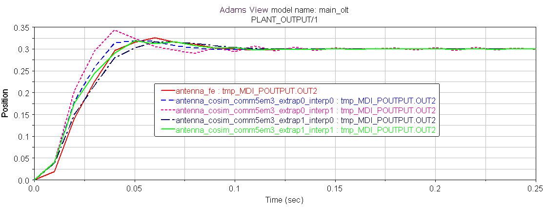
Plot of control torque: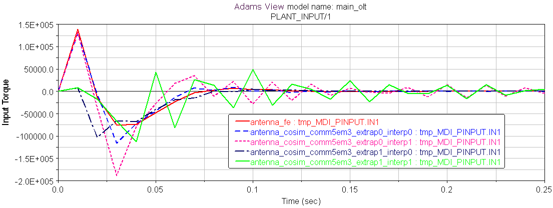
Thus, linear extrapolation can help get an accurate answer, as long as the communication interval is small enough to provide an accurate prediction.