Example of Working with a Preloaded Flexible Body
Overview
In this example, you’ll explore how the behavior of flexible bodies changes when they correspond to a deformed configuration. The example does not address how you would create such a flexible body description because this varies depending on the FEA program with which you are working.
This example illustrates the behavior of preloaded flexible bodies using two links shown in Figure 7. Both links correspond to the same physical component, but one has been stretched by 1E+7N axial force. During the simulations, you’ll discover how the behavior of the stretched link is different from the undeformed link. In addition, you’ll discover how the behavior of the link changes when it is constrained.
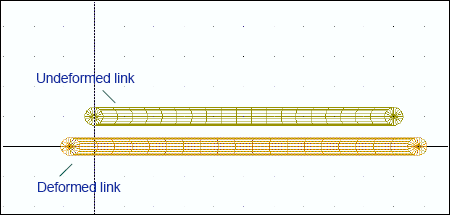
Figure 7 Undeformed and Deformed Links
Starting Adams View
You’ll start the example by running Adams View and creating a new model.
To start Adams View and create a database for the flexible body:
1. Copy the file link.mnf and deflink.mnf to your local directory. This file is located in install_dir/flex/examples/mnf, where install_dir is the directory where the Adams software is installed.
2. Start Adams View and create a new model, named links, that has no gravity. Use the default units.
Integrating the Links
Now you’ll integrate the MNFs containing the links.
To import the links:
1. Import link.mnf into your model using the default damping ratio. Name the flexible body UNDEFORMED.
A link appears.
2. Turn on the working grid.
3. Move UNDEFORMED up by one grid space.
4. Import deflink.mnf into your model using the default damping ratio. Name the flexible body DEFORMED.
You’ve now created two flexible bodies. Both bodies correspond to the same physical component, but one has been stretched by a 1E-7N axial force.
Simulating the Preloaded Flexible Bodies
You’ll now perform a static equilibrium simulation on the two bodies. A static simulation attempts to find a configuration for the bodies for which all the forces balance.
To perform a static equilibrium simulation:
1. Click the Simulation tab. From the Simulate container, select Simulate  .
.
. 2. Select the Static Equilibrium tool. .
.
.As you would expect, the stretched flexible body recoils to its undeformed configuration because the load that caused the body to be deformed is no longer present.
You also see color contours on DEFORMED. They show how the body deforms relative to its input configuration.
Adding Joints to Deformed Body
You’ll now add two revolute joints to DEFORMED. During a simulation, the load built into DEFORMED is transferred to these joints.
To add joints:
1. Return the model to its input configuration.
2. Add revolute joints to nodes 1000 and 1001 of DEFORMED. Node 1000 is at the left end of the flexible body and Node 1001 is at the right end.
Tip: | If you have trouble selecting the nodes, try zooming in on the model by pressing the letter w and drawing a zoom window. Then right-click to display a list of nodes near your cursor. |
Performing Simulation and Investigating Results
You’ll now perform a dynamic simulation and investigate the results of the simulation in Adams PostProcessor to see that the 1E-7N load that was built into DEFORMED has been transferred to the joints you created.
To perform a simulation and investigate results:
1. Perform a dynamic simulation for 1 second with 50 steps.
2. From the Review menu, select PostProcessing.
Adams PostProcessor appears.
3. From the Filter list, select constraint.
4. From the Object list, select both joints.
5. From the Characteristic list, select Element_Force.
6. From the Component list, select X, and then select Add Curves.
Note that although the color contours indicate a deformation, they are displaying numerical noise.