Modal Superposition
The single most important assumption behind the FLEX_BODY is that we only consider small, linear body deformations relative to a local reference frame, while that local reference frame is undergoing large, non-linear global motion.
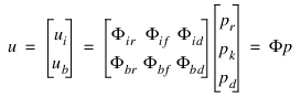
The discretization of a flexible component into a finite element model represents the infinite number of DOF with a finite, but very large number of finite element DOF. The linear deformations of the nodes of this finite element mode,  , can be approximated as a linear combination of a smaller number of shape vectors (or mode shapes),
  .
.
, can be approximated as a linear combination of a smaller number of shape vectors (or mode shapes), .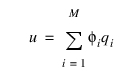 | (7) |
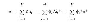
where  is the number of mode shape. The scale factors or amplitudes,
  , are the modal coordinates.
is the number of mode shape. The scale factors or amplitudes, , are the modal coordinates. As a simple example of how a complex shape is built as a linear combination of simple shapes, observe the following illustration:
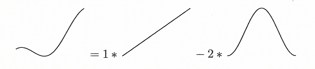
Figure 2 Complex shape built as a linear combination of simple shapes
The basic premise of modal superposition is that the deformation behavior of a component with a very large number of nodal DOF can be captured with a much smaller number of modal DOF. We refer to this reduction in DOF as modal truncation.
Equation (7) is frequently presented in a matrix form:
 | (8) |
where  is the vector of modal coordinates and the modes
  have been deposited in the columns of the modal matrix,
  . After modal truncation
  becomes a rectangular matrix. The modal matrix
  is the transformation from the small set of modal coordinates,
  , to the larger set of physical coordinates,
  .
.
is the vector of modal coordinates and the modes have been deposited in the columns of the modal matrix, . After modal truncation becomes a rectangular matrix. The modal matrix is the transformation from the small set of modal coordinates, , to the larger set of physical coordinates, . This raises the question: How do we select the mode shapes such that the maximum amount of interesting deformation can be captured with a minimum number of modal coordinates? In other words, how do we optimize our modal basis?
Component Mode Synthesis (CMS)
Adams is capable of taking in modes that generated from different kinds of CMS methods. In general, the component modes are generated by the Ritz approach in which a truncated set of normal modes is combined with particular static modes. The type of normal modes, either free or constrained, and the type of static modes characterize and distinguish a CMS method from another [1-2]. Standard modal reduction, Craig-Bampton method and Craig-Chang method are briefly recalled here but Adams is not limited to these modal bases.
Standard modal reduction
If the flexible body i is assumed to vibrate freely with respect to its reference, one has
 | (9) |
where,  is the assembled matrix of the element
  matrices. The stiffness matrix
  is positive definite, because of imposing the reference conditions that define a unique displacement field.
is the assembled matrix of the element matrices. The stiffness matrix is positive definite, because of imposing the reference conditions that define a unique displacement field.This equation can be used to determine the mode shapes (assumed modes of displacements). The mode shapes can be used to form the modal matrix  , which has a number of columns nf equal to the number of elastic nodal coordinates of the flexible body. A reduced order model can be achieved by solving only for nm mode shapes. A coordinate transformation from the physical nodal coordinates to the modal elastic coordinates using nm modes can be written as,
, which has a number of columns nf equal to the number of elastic nodal coordinates of the flexible body. A reduced order model can be achieved by solving only for nm mode shapes. A coordinate transformation from the physical nodal coordinates to the modal elastic coordinates using nm modes can be written as, | (10) |
where  is the modal transformation matrix, whose columns are the selected nm fundamental mode shapes, and
  is the nm -vector of modal coordinates.
is the modal transformation matrix, whose columns are the selected nm fundamental mode shapes, and is the nm -vector of modal coordinates.The reference and elastic generalized coordinates are written in terms of the reference and modal coordinates as,
 | (11) |
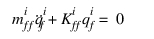
The equations of motion for the flexible body i expressed in modal coordinates can be written as,
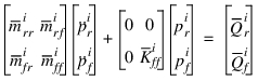
where the generalized mass and stiffness matrix corresponding to the reduced modal coordinates are,
 | (12) |
 | (13) |
Note that since the reference conditions are used to eliminate the rigid body modes, the reference and elastic inertia coupling terms presented in Equation (12) are no longer zero values.
The Craig-Bampton method
Capturing the effects of attachments on the flexible body in a dynamic system simulation can be difficult for many modal reduction techniques in achieving model fidelity. For example, using only normal modes often required an excessive number of modes. Using only these modes as eigenvectors were found to provide an inadequate basis in system level modeling due to modal truncation.
The solution was to use Component Mode Synthesis (CMS) techniques, and the most general methodology is the Craig Bampton method. Note that there is some ongoing research that recommends reference conditions are to be applied to the finite element model before carrying out the Craig-Bampton method in order to ensure a unique displacement field for the dynamic system simulation [3].
The Craig-Bampton method allows the user to select a subset of DOF which are not to be subject to modal truncation. These DOF, which we refer to as boundary DOF (or attachment DOF or interface DOF), are preserved exactly in the Craig-Bampton modal basis. There is no loss in resolution of these DOF when higher order normal modes are truncated.
The Craig-Bampton method achieves this with a very simple scheme. The system DOF are partitioned into boundary DOF,  , and interior DOF,
  . Two sets of mode shapes are defined, as follows:
, and interior DOF, . Two sets of mode shapes are defined, as follows: ■Constraint modes: These modes are static shapes obtained by giving each boundary DOF a unit displacement while holding all other boundary DOF fixed. The basis of constraint modes completely spans all possible motions of the boundary DOFs, with a one-to-one correspondence between the modal coordinates of the constraint modes and the displacement in the corresponding boundary DOF,  .
.
.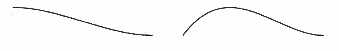
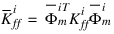
Figure 3 Two constraint modes for the left end of a beam that has attachment points at the two ends.
The figure on the left shows the constraint mode corresponding to a unit translation while the figure on the right corresponds to a unit rotation.
■Fixed-boundary normal modes: These modes are obtained by fixing the boundary DOF and computing an eigen solution. There are as many fixed-boundary normal modes as the user desires. These modes define the modal expansion of the interior DOF. The quality of this modal expansion is proportional to the number of modes retained by the user.
Figure 4 Two fixed-boundary normal modes for a beam that has attachment points
at the two ends.
at the two ends.
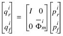
The relationship between the physical DOF and the Craig-Bampton modes and their modal coordinates is illustrated by the following equation.
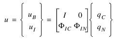 | (14) |
where:
 | = | the boundary DOF. |
 | = | the interior DOF. |
 | = | identity and zero matrices, respectively. |
 | = | the physical displacements of the interior DOF in the constraint modes. |
 | = | the physical displacements of the interior DOF in the normal modes. |
 | = | the modal coordinates of the constraint modes. |
 | = | the modal coordinates of the fixed-boundary normal modes. |
The generalized stiffness and mass matrices corresponding to the Craig-Bampton modal basis are obtained via a modal transformation. The stiffness transformation is:
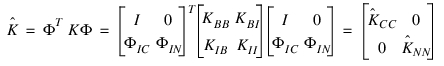 | (15) |
while the mass transformation is:
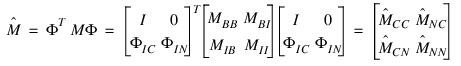 | (16) |
where the subscripts  ,
,  ,
,  , and
, and  denote internal DOF, boundary DOF, normal mode and constraint mode, respectively. The caret on
  and
and  denotes that this is generalized mass and stiffness.
, , , and denote internal DOF, boundary DOF, normal mode and constraint mode, respectively. The caret on and denotes that this is generalized mass and stiffness. Equation (15) and Equation (16) have a few noteworthy properties:
■ and
and  are diagonal matrices because they are associated with eigenvectors.
and are diagonal matrices because they are associated with eigenvectors.■ is block diagonal. There is no stiffness coupling between the constraint modes and fixed-boundary normal modes.
is block diagonal. There is no stiffness coupling between the constraint modes and fixed-boundary normal modes.■Conversely,  is not block diagonal because there is inertia coupling between the constraint modes and the fixed-boundary normal modes.
is not block diagonal because there is inertia coupling between the constraint modes and the fixed-boundary normal modes.The Craig-Chang method
Unlike Craig-Bampton method that utilize fixed-interface modes, there exists other model CMS techniques that consists of free-interface modes, rigid-body modes and residual inertia relief attachment modes. This is known as Craig-Chang method which is detailed in reference [4].
The free-interface modes are simply the structure modes if the boundary or interface degrees of freedom are unconstrained. These modes can be computed by solving the eigenproblem for the full mass matrix and the full stiffness matrix in the following free-vibration equations.
 | (17) |
One could use  to denote the free-interface modes that corresponds to the eigenfrequency
  .
.
to denote the free-interface modes that corresponds to the eigenfrequency .The rigid-body modes can be obtained by setting  and this leads to
  , where
  represents the set of rigid-body modes.
and this leads to , where represents the set of rigid-body modes.The residual inertia relief attachment modes are obtained by giving each boundary DOF a unit force while holding all other boundary DOF fixed and these modes are linked to the residual flexibility matrix  .
.
. | (18) |
Using the same partition between internal and boundary degrees of freedom as Equation (14) and drop the body index i for simplicity the transformation between physical coordinates and Craig-Chang modal coordinates can be obtained as,
 | (19) |
where the subscript i represents the internal DOFs and b represents the boundary DOFs. And the reduction transformation matrix Φ is then applied to the mass and stiffness matrix to reduce them into the Craig-Chang formulation as below,
 | (20) |
Mode Shape Orthonormalization
CMS is a powerful method for tailoring the modal basis to capture both the desired attachment effects and the desired level of dynamic content. However, the raw CMS modal basis has certain deficiencies that make it unsuitable for direct use in a dynamic system simulation.
1. The CMS modes are not an orthogonal set of modes, as evidenced by the fact that their generalized mass and stiffness matrices  and
and  , encountered in Equation (15) and Equation (16), are not diagonal.
and , encountered in Equation (15) and Equation (16), are not diagonal. 2. Constraint modes are the result of FE static condensation. Consequently, these modes do not advertise the dynamic frequency content that they must contribute to the flexible body. Simulation of a non-linear system with unknown frequency content can lead to unexpected results
3. The modes embedded in the CMS method may have up to 6 rigid body DOF which must be eliminated before the dynamic system simulation because Adams provides its own large-motion rigid body DOF as flexible body states in the analysis.
The problems with the raw CMS modal basis are all resolved by applying a simple mathematical operation on the CMS modes called orthonormalization. Note that mode shape orthonormalization is two phased, one is orthogonalization and then, mass normalization of the CMS modes. The process of modal shape orthogonalization is recalled next.
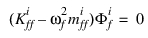
By solving an eigenvalue problem:
 | (21) |
we obtain eigenvectors that we arrange in a transformation matrix  , which transforms the CMS modal basis to an equivalent, orthogonal basis with modal coordinates
  :
:
, which transforms the CMS modal basis to an equivalent, orthogonal basis with modal coordinates : | (22) |
The effect on the superposition formula is:
 | (23) |
where  are the orthogonalized CMS modes.
are the orthogonalized CMS modes.The orthogonalized CMS modes are not eigenvectors of the original system. They are eigenvectors of the CMS representation of the system and as such have a natural frequency associated with them. In addition, these eigenvectors span the same modal basis as the raw CMS modes. A physical description of these modes is difficult, but in general the following is observed:
■Fixed-boundary normal modes are replaced with an approximation of the eigenvectors of the unconstrained body. This is an approximation because it is based only on the CMS modes. Out of these modes, 6 modes are usually the rigid body modes.
■Constraint modes are replace with boundary eigenvector, a concept best illustrated by comparing the modes before and after orthogonalization of a rectangular plate which has CMS attachment points along one of its long edges. The CMS mode in Figure 5 features a unit displacement or force of one of its edge nodes with all the other nodes along that edge fixed. After orthonormalization we see modes like the one depicted in Figure 6, which has a sinusoidal curve along the boundary edge.
■Finally, there are modes in a gray area between the first two sets that defy physical classification.
We conclude that the orthogonalization of the CMS modes addresses the problems identified earlier, because:
1. Orthogonalization yields the modes of the unconstrained system. These are free-free modes, 6 of which are rigid body modes, which can now be disabled.
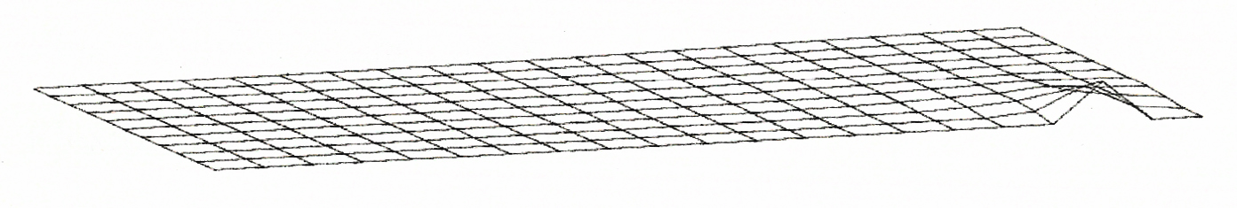
Figure 5 Constraint mode with an unknown frequency contribution.
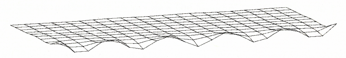
Figure 6 Boundary eigenvector with a 1250 Hz natural frequency.
2. Following the second eigensolution, all modes have an associated natural frequency. Problems arising from modes contributing high-frequency content can now be anticipated.
3. Although the removal of any mode constrains the body from adopting that particular shape, the removal of a high-frequency mode such as the one depicted in Figure 6 is clearly more benign than removing the mode depicted in Figure 5. The removal of the latter mode prevents the associated boundary node from moving relative to its neighbors. Meanwhile, the removal of the former mode only prevents boundary edge from reaching this degree of “waviness.”
Note that CMS modes should not be disabled after orthogonalization because one might remove a constraint mode which may numerically stiffen the flex body system.
References
1. R.J. Guyan, Reduction of stiffness and mass matrices, AIAA J. 3 (2) (1965) 380
2. A.Y.-T. Leung, An accurate method of dynamic condensation in structural analysis, Int. J. Numer. Meth. Eng. 12 (11) (1978) 1705–1715.
3. A. Cammarata and C.M. Pappalardo, On the use of component mode synthesis methods for the model reduction of flexible multibody systems within the floating frame of reference formulation, Mechanical Systems and Signal Processing. Vol 142 (2020), 10675.
4. R.R. Craig and C-J Chang, On the use of attachment modes in substructure coupling for dynamic analysis, Paper 77-405, AIAA/ASME 18th Structures, Structural Dynamics , and Material Conference, San Diego , CA 1977.