Gear Pair - Mass (Advanced 3D Contact)
Machinery → Create Gear Pair
By default, Adams View calculates the mass and inertia for a rigid body part based on the part's geometry and material type. The geometry defines the volume and the material type defines the density. The default material type for rigid bodies is steel.
You can change the material type used to calculate mass and inertia or simply specify the density of the part. If you do not want Adams View to calculate mass and inertia using a part's geometry, material type, or density, you can enter your own mass and moments of inertia.
It is possible to assign zero mass to a part whose six Degrees of freedom you constrain with respect to parts that do have mass. You should not assign a part zero mass, however. Any part that has zero mass and translational degrees of freedom can causes simulation failure (since a = F/m). Therefore, we recommend that you assign finite masses and inertias to all parts. In addition, a part without mass cannot have mass moments of inertia.
Learn about Methods for Calculating Mass Properties.
For the option | Do the following |
|---|---|
Material (Gear1/Gear2) | |
Define Mass By | ■User Input If you do not want Adams View to calculate mass and inertia using a part's geometry, material type, or density, you can enter your own mass and moments of inertia. ■Geometry and Density You can change the material type used to calculate mass and inertia or simply specify the density of the part. ■Geometry and Material Type The geometry defines the volume and the material type defines the density. |
If you select User Input, the following options will be displayed: | |
Mass | Enter the mass of the gear part. |
The parts are located at the center of the gear, with the z-axis as the rotational axis. | |
Inertia | |
Ixx/Iyy/Izz | Enter the values that define the principal mass-inertia components of the gear part. |
Ixy/Izx/Iyz | Enter the values that define the deviational (cross-product) mass-inertia components of the gear part. |
Young’s Modulus | Young's modulus E defines the relation between tensile strain  and tensile stress and tensile stress  by Hooke's law: by Hooke's law:  |
Poisson’s Ratio | An extension  of a linear elastic and isotropic material is accompanied by lateral strains of a linear elastic and isotropic material is accompanied by lateral strains  and and  . Poisson's ratio . Poisson's ratio  defines this relation by equations: defines this relation by equations:   Or  where G is shear modulus. where G is shear modulus. |
Material Density | The mass m of a solid body is computed by equation its volume V multiplied by the mass density  . .  |
If you select Geometry and Density, the following options will be displayed: | |
Density | Enter the density value. |
Young’s Modulus | Young's modulus E defines the relation between tensile strain  and tensile stress and tensile stress  by Hooke's law: by Hooke's law:  |
Poisson’s Ratio | An extension  of a linear elastic and isotropic material is accompanied by lateral strains of a linear elastic and isotropic material is accompanied by lateral strains  and and  . Poisson's ratio . Poisson's ratio  defines this relation by equations: defines this relation by equations:   Or  where G is shear modulus. where G is shear modulus. |
If you select Geometry and Material Type, the following options will be displayed: | |
Material Type | Enter the material type to be used inertia calculation. |
Density | Enter the density value. |
Young’s Modulus | Young's modulus E defines the relation between tensile strain  and tensile stress and tensile stress  by Hooke's law: by Hooke's law:  |
Poisson’s Ratio | An extension  of a linear elastic and isotropic material is accompanied by lateral strains of a linear elastic and isotropic material is accompanied by lateral strains  and and  . Poisson's ratio . Poisson's ratio  defines this relation by equations: defines this relation by equations:   Or  where G is shear modulus. where G is shear modulus. |
Contact Settings Note: To get a full description of all contact parameters please refer to the online help for the IMPACT function. | |
Modeling Options | ■Rigid Gear ■RunTime ■PreComputed |
If Rigid Gear selected, the following options will be displayed: Uses an advanced surface-to-surface contact algorithm, which delivers accurate and smooth results. The algorithm considers changing shaft positions and misalignment. The tooth flanks are described by the extruded profile including the micro-geometry. The solids for display are not used for the contact computation. The contact is checked for the left and right flanks of 5 tooth pairs. | |
Contact Stiffness | For Rigid Gear body contact, the maximum penetration of each contact plane of gear_1 into the flank of gear_2 is used for the calculation of the corresponding contact force Fcnt as shown by equation: Fcnt = k * penec_exp where: ■k = contact stiffness ■pene = maximum penetration ■c_exp = exponent force law The vector sum of all contact forces is giving the resulting contact forces and torque per gear stage. |
Stiffness Exponent | In general, the deformation of a tooth is coming from the deformation of the wheel body, the deformation of the teeth and the Hertz contact. The contribution of the Hertz contact is limited compared to the two other contributions. Consequently one has to assume, that the stiffness exponent is close to 1 or only slightly higher. An exponent of 1 corresponds to a linear contact stiffness. |
If RunTime selected, the following options will be displayed: Uses an advanced surface-to-surface contact algorithm, which delivers accurate and smooth results. The algorithm considers changing shaft positions and misalignment. The tooth flanks are described by the extruded profile including the micro-geometry. The solids for display are not used for the contact computation. The contact is checked for the left and right flanks of 5 tooth pairs. | |
Contact Overlap | Transmitted force between tooth flanks considers the flexibility of the teeth through the solution of a non-linear contact problem. The contact algorithm is of type surface-to-surface. A small relaxation by 'contact overlap' is introduced for better performance. Supported values are Small, Normal or High. Small corresponds to stiffer. The effect of this additional flexibility is small compared to the flexibility of the teeth. |
If PreComputed selected, the following options will be displayed: Offers pre-computed contact formulation delivering high performance with good results quality. In this method damping and friction are computed with simplified methods. The relative velocities in contact are evaluated only in middle plane of gear wheels. This approach can lead to noisy results under dynamic simulations; therefore adjustments for damping should be made with caution. The Friction model is reduced to 2 parametric model, with one friction coefficient and one threshold velocity. | |
GCP File Name | Select created GCP file containing pre-computed contact data with Browse option. |
Tooth Profile | User can create profile through the standard rack definition of the manufacturing process. The relevant profile data is transferred to the DAT-File, which is used for the simulation. When user enters the manufacturing data for rack definition, he can preview the gear profile on gear setting page as shown below: |
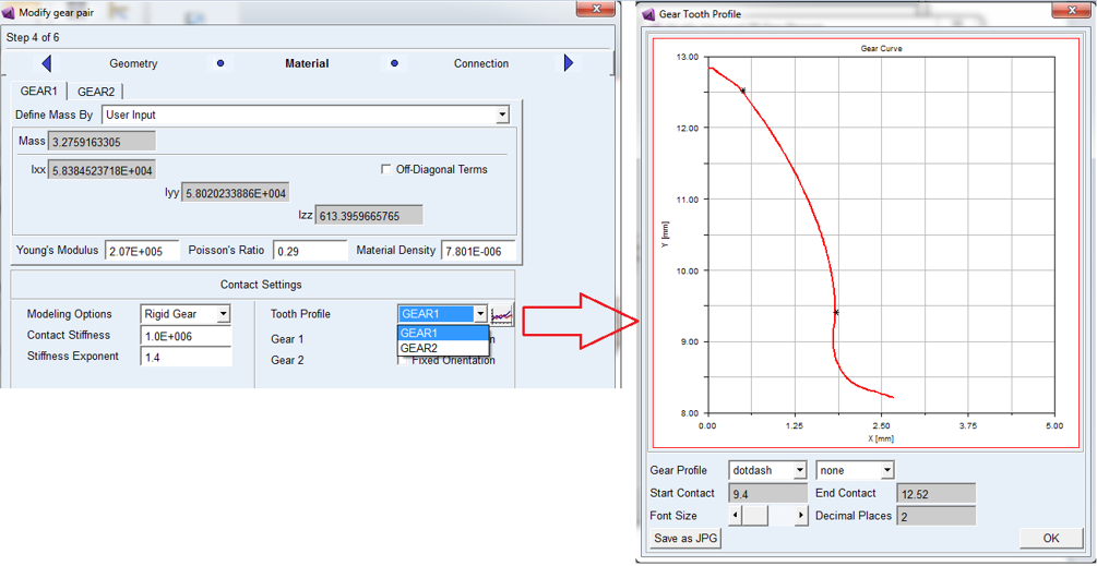 | |
Fixed Orientation | The toggle fixed orientation defines the gear wheel, which is fixed for the assembly while meshing the gears. The gears are meshed at the time of force creation so that the teeth fit exactly into the design position, which should show a clearance between the teeth flanks. An internal gear will always be the reference (fixed) gear and the external gear will be rotated. In case of planetary, consequently, the planet(s) will have fixed orientation with respect to the sun. Following rules are applicable: ■At least one gear must be an external one ■The internal gear must be Gear 2 ■Gear 1 is automatically the wheel with smaller width in case of two external gears |
Friction Model | ■On ■Off |
Static Coefficient | The static friction coefficient is usually higher than the dynamic friction coefficient. |
Slip Velocity | 'slip velocity' limits the region of sign change of the sliding velocity. The combination of very small slip velocity and high friction can reduce the performance of the integrator. The user is advised to validate his selection through post-processing of the sliding velocity. |
Dynamic Coefficient | The dynamic friction coefficient is usually smaller than the static friction coefficient. |
Transition Velocity | Transition velocity defines the start of the region, where the dynamic friction is constant. |
Clearance Check | Checks the clearance in the gear stage by using the shells geometries (solid) of the gear rim. If clearance - what should be the normal case - is found, it will be shown as depicted in figure. The gear solids do not include the micro-geometry. 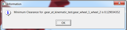 |
Force Verify  | This creates and loads automatically an Adams model with the name verify_gear_AT_model. This model allows a visual check of the profiles of the gear stage. The filled areas represent the portion of the profile between start contact and end contact. 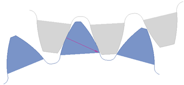 |
Damping Oil Rate Oil Film Thickness | The effects of hydrodynamic damping depend on gap height and squeeze velocities. The implemented damping force defined through 'damping rate oil' approximates hydrodynamic damping in function of the gap for each contact plane between the tooth flanks and the corresponding squeeze velocity. The function b is used to define the damping: b = 1.0 - gap / ( 2 * oil film thickness ) There is no hydrodynamic damping, when b < 0 Fhyd = 0 for b < 0 Hydrodynamic damping increases exponentially with decreasing oil film height. The introduction of the damping exponent d_exp is used for this purpose: Fhyd = damp rate oil * squeeze vel * bd_exp for 0 < b < 1 In case of contact (penetration), the hydrodynamic damping force is set as shown by equation: Fhyd = damp rate oil * squeeze vel for b > 1 The damping rate has always to be entered in units [N*s/mm] in this release. 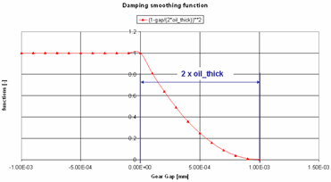 Hydrodynamic damping |
Damping Rate Structure Damping Exponent | Structural damping is usually a small value. The structural damping force is made proportional to the contact force as shown by equation: Fstruc_damp = Fcnt * damp structure * sign (squeeze vel) A value of 0.01 means that the structural damping force is 1 percent of the elastic contact force. Friction is computed for each contact plane of 'gear_1' based on the relative sliding velocity at the contact point. |
Transient Damping Damping Rate End Time | ■On ■Off Transient damping influence the resulting contact torque component about the rotational axis. Its purpose is to reduce time needed to overcome initial transient phase in dynamic simulation. The damping is proportional to angular velocity difference of ideal gear pair relative to existing one. The coefficient of proportionality and the time the damping is active can be set. The damping torque is determined with formula: delta_omega = omega_w1 - omega_w2 * N2 / N1 Tdam = delta_omega * Damping_Rate Friction effects can be turned On/Off through the toggle friction model. The static friction coefficient is usually somewhat higher than the dynamic friction coefficient. Step functions are used for smoothing the transitions. The slip velocity limits the region of sign change of the sliding velocity. The combination of very small slip velocity and high friction can reduce the performance of the integrator. You are advised to validate your selection through post-processing of the sliding velocity. Transition velocity defines the start of the region, where the dynamic friction is constant. 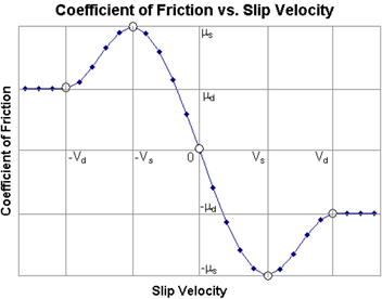 |