Adams View - Setup and run Ball and Beam model
Overview
This tutorial will guide you through the process of creating control system, transducer signals, actuator signal, connect the signals and run a simulation. For this tutorial the ‘ball and beam’ example model delivered with standard Adams Controls will be used as a base. The control system will later on uses the code generated from MATLAB/Simulink.
The main steps covered in this tutorial are:
Open and review the base model
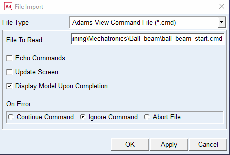
Copy the tutorial directory <install_dir>/amech/examples/aview/tutorial_ball_beam to your working directory. Start Adams View, and select the just created directory as working directory and import the Adams command file ball_beam_start.cmd to load the model.
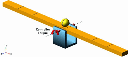
This is a model of a ball rolling on a beam and the position of the ball will be controlled by a control system torque applied in the pin joint attaching the beam to the ground.
Create the Control System
In this tutorial we will start with creating the control systems however, alternatively we could as well have started by creating the transducer and actuator signals.
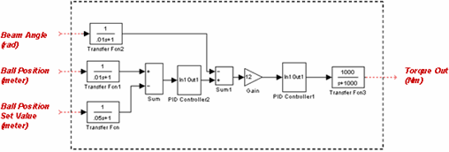
First we will create the regulator control systems. The MATLAB/Simulink model is shown with the required angle and positions input and the produced torque output. Alternatively the model can be created in Easy5.
Then we create a control system in Adams Mechatronics. Load the Mechatronics plugin if it is not already loaded:
Tools → Plugin Manager → Adams Mechatronics → Load (Yes) → OK
Next, create the Control System:
Mechatronics → Control System → New
Fill in the dialog box as you see below, and then select the  icon to start the Control Signal Editor.
icon to start the Control Signal Editor.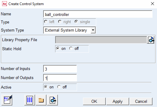
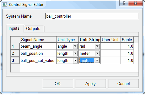
Control Signal Editor is used to define the Control Signal Inputs/Outputs specification such as Name, Unit Type, Unit String. Fill in the three controlsignal input names, unit type, and unit string as depicted below.
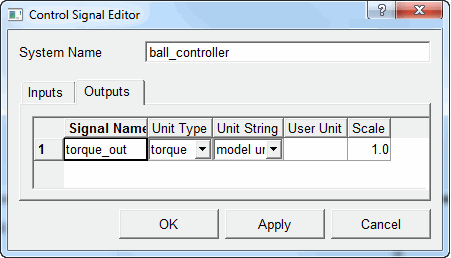
And then the control signal output specification as shown in next picture.
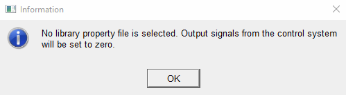
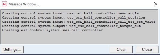
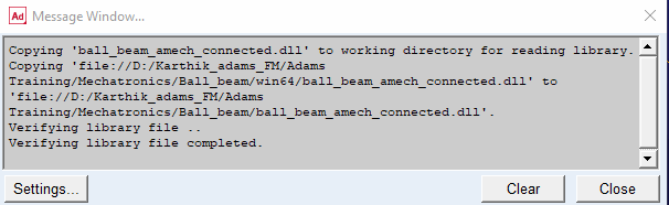
Then select OK in Control Signal Editor dialog box to close the dialog box and return to the Create Control System dialog box, where you select OK button again. The following Message Window informs you that the control system output signals will be set to zero since no property file was selected.
Close the dialog box by selecting the OK button. The following Message Window appears to verify that the control system with given specification are created. You can close the Message Window.
Create the Transducer Signals
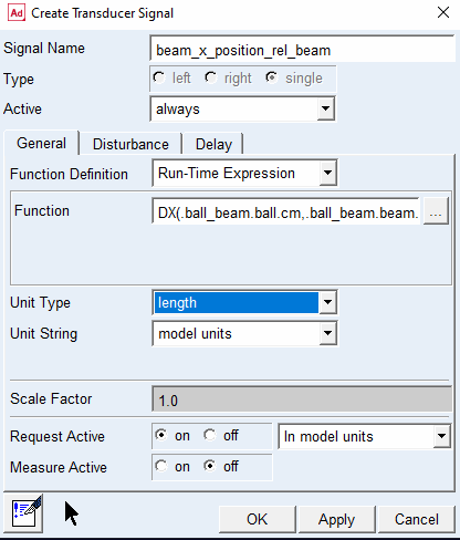
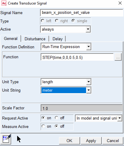
Now you create the appropriate transducers so that you can connect the mechanical system to the control system, by using the menu Mechatronics → Mechanical System → Transducer Signal → New
Start with creating the transducers as the following pictures show. Here you may take advantage of the Function Builder by selecting  icon to build the function expression. Make sure to activate the requests for all three transducers.
icon to build the function expression. Make sure to activate the requests for all three transducers.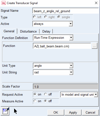
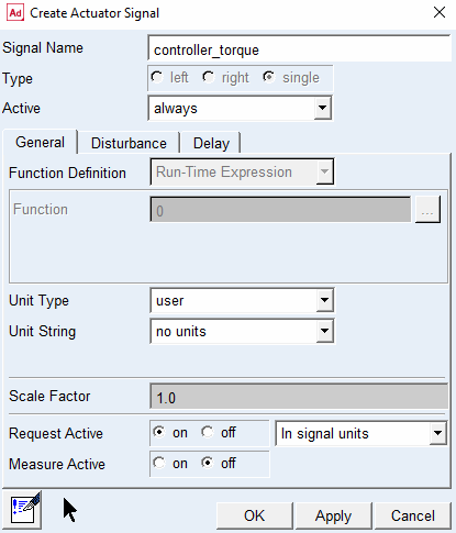
Create the Actuator Signal
Next you create an actuator signal using the menu Mechatronics → Mechanical System → Actuator Signal → New
You do not need to choose a function for actuator signal of controller_torque as its value is fed by the control system. Also note that for all signals so far, we have niether applied any disturbance nor any delay.
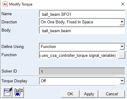
Applying the Control System
Now you need to modify the torque function which is applied to beam so that it gets its value from the actuator. To modify the torque, double-click the background of the Adams View main window to clear any selections. From the Edit menu, select Modify which shows the Database Navigator. Then select the torque as shown below.
Connect Signals with Signal Manager
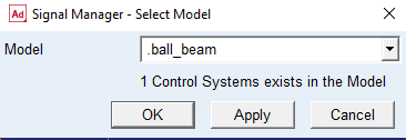
Next you start the Signal Manager from Mechatronics → Signal Manager → Display
Select the Apply button, with the shown model to see the control system.
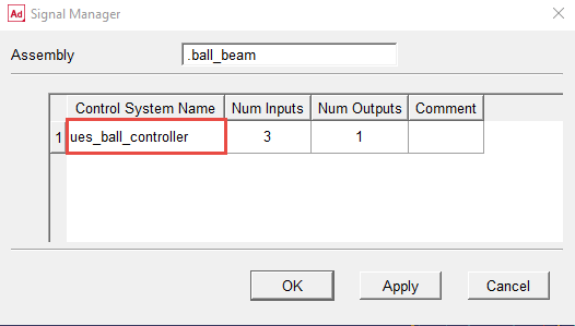
Double-click any cell of the control system in the table to select the control system of interest.
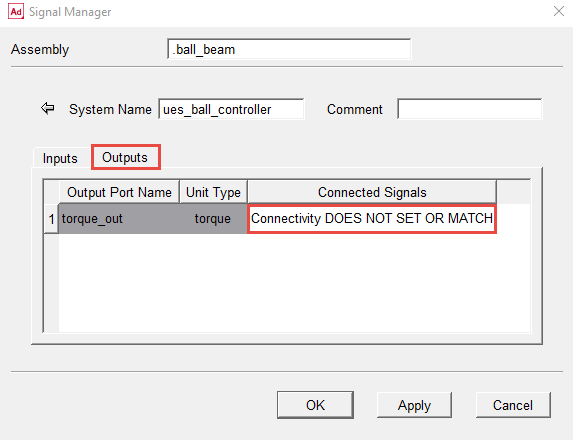
As can be seen from the following picture, no signal is connected to the input ports of the controller, that is, Connectivity is NOT SET.
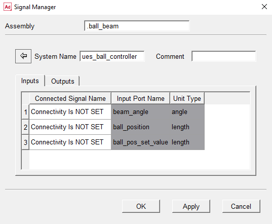
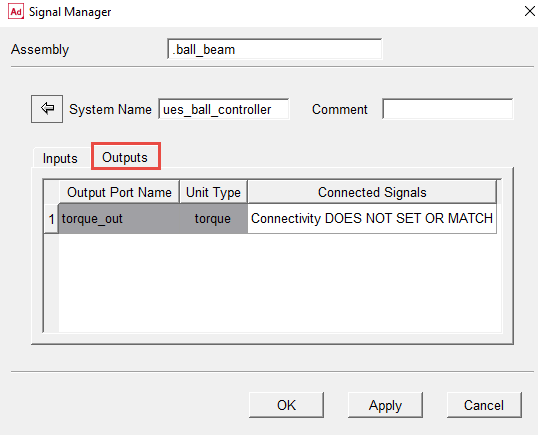
Neither any signal is connected to the output port.
You can select and connect appropriate signals by double-clicking on any cell of interest that has a white background. For instance, start with a double-click on the first cell under the connected signal name in the inputs list. The Selecting Input… dialog box pops up.
As you see, there is only one signal of unit type of Angle in Available Signal List. You select this signal to be connected the input port of beam angle by clicking on one of the corresponding cells in the table, and consequently selecting the select button in the lower-left area of the dialog box.
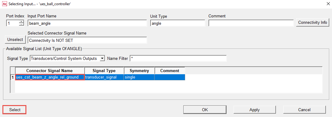
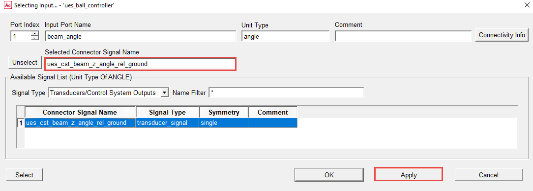
Upon selecting the select button, the transducer signal name will appear in Selected Connector Signal Name. Select Apply to save the selection. Note that when a selection is saved, the corresponding row in the Available Signal List table gets a blue background color.
Now by changing Port Index counter, review the next input port, that is, ball_postion.
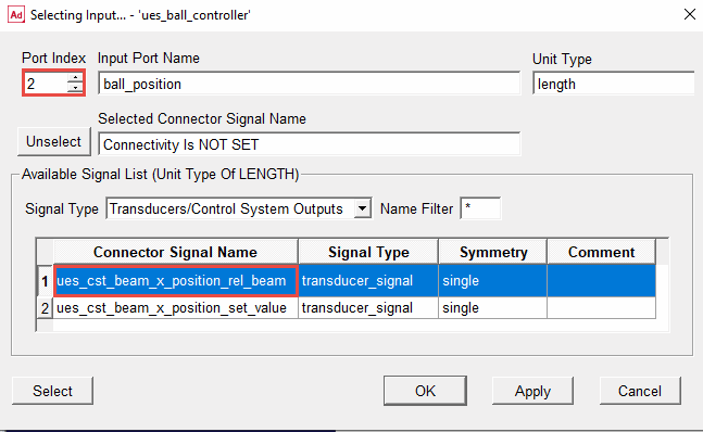
As there are two signals of unit type of Length which can be seen in the Available Signal List table, you should select the ues_cst_ball_x_position_rel_beam transducer signal by double-clicking on one of the corresponding cell in the table. Note that after selection by double-clicking, you have automatically guided to the next (third) input port.
Tip: | Double-clicking in this table is short cut for selecting the signal, selecting the Apply button, and going to the next port. |
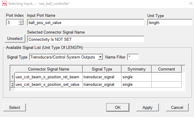
In the third input port, select the ues_cst_ball_x_position_set_value by clicking in a cell in the corresponding row, clicking the select button, and then selecting the OK button to both confirm the selection and close the Selecting Input … dialog box in the same time.
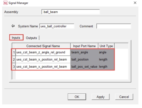
Now you are back again in the page that you could review the input/output ports. As you see now all the input ports are connected to appropriate transducer signals.
Similarly, you navigate to the output port side by selecting the Outputs tab and then by double-clicking the connected signal cell (white area) in the table, you go to the Selecting Output … dialog box.
Similarly, select the controller_signal to be connected to output port of the controller.
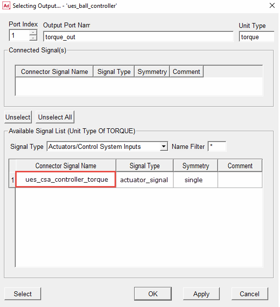
As a result, the selected actuator signal will show up in the connected signal(s) list. Click OK to confirm the selection and close this dialog box.
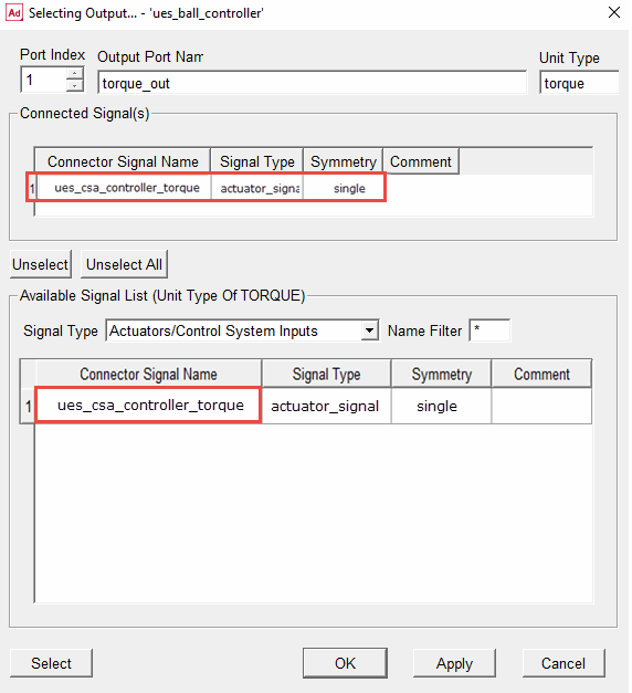
Now you can see that the torque_out output port is connected to controller_torque actuator signal.
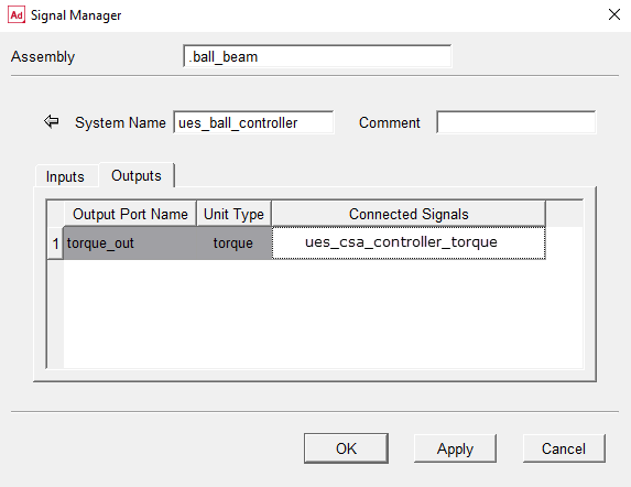
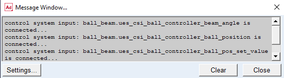
Select OK to confirm all selection you have done in the signal manager. The following message windows reports the connection made.
Export Plant
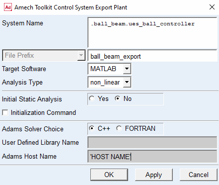
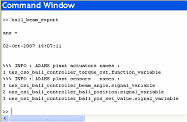
You now export the plant in order to create the External System Library (ESL) file in MATLAB/Simulink or Easy5. Go to the Mechatronics → Tools → Export Plant
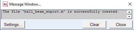
Fill out the dialog box as shown below. In particular, select a File Prefix (in this case, ball_beam_export), verify the control System Name and Target Software have chosen correctly, and keep the default values for other parameters. Finally, select OK; the message window confirms that the MATLAB file ball_beam_export.m, or Easy5 ball_beam_export.inf has been successfully created.
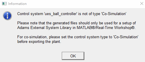
Since this is an External System Library system, you will see this message:
Create the MATLAB/Simulink External System Library
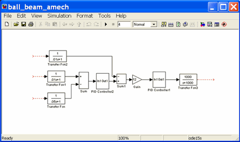
Now Start the MATLAB/Simulink and open the model ball_beam_amech.mdl which is provided in the example directory. Read in the file ball_beam_amech_param.m to set the PID parameters for the two PID-Controllers.
Read in the exported plant file ball_beam_export.m. The following message appears.
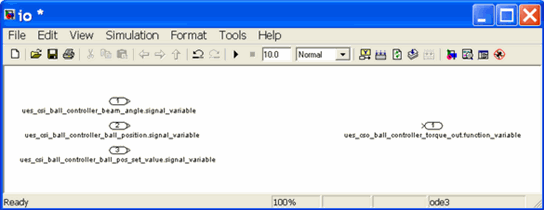
Enter setio to generating the input and output ports in MATLAB/Simulink as depicted below.
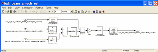
You now merge the two models (ball_beam_amech.mdl and the io model) by connecting the signal and then save the model as ball_beam_amech_esl. The model should look like below.
Follow the instructions on how to generate the ESL file in standard Adams Controls. In particular, you need to setup the Adams files for Code Generation by manually running process.py or using the command setup_rtw_for_adams which will do this for you. Do not forget to verify that the PID parameters are defined as inline parameters (that is, tunable parameters).
Create Easy5 External System Library (optional alternative to MATLAB ESL)
Copy the files from <install_dir>/amech/examples/ball_beam/easy5 into your working directory. The file from the Mechatronics Plant Export need to be in the same directory as the Easy5 model.
Start Easy5 in your working directory and open the model ball_beam.0.ezmf. Double click on the Adams block and go to the Documentation/Configuration tab. Click on Select/Configure Adams model
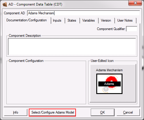
Select the exported plant file and choose Function Evaluation - No Feed through as the simulation mode. Click Done in this dialog box and OK in the AD- Component Data Table dialog box to apply these changes.
Now, go to the Build menu to create the External System Library
Build → Export Model As →ADAMS External System Library…
The following dialogbox is displayed:
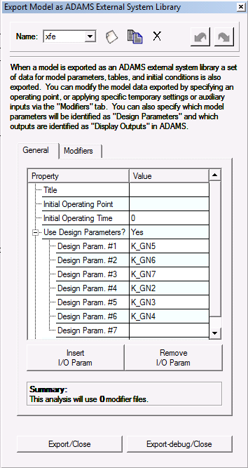
To expose the PID gains as design variables in Adams View, change Use Design Parameters to Yes, and select gains K_GN2, K_GN3, K_GN4, K_GN5, K_GN6, and K_GN7 from the PID controller submodels.
Select Export/Close in this dialog box to create the ESL (that is, ball_beam.dll on Windows and ball_beam.so on Linux) and supporting ball_beam.xfe.ezanl file.
Generate ESL Property File
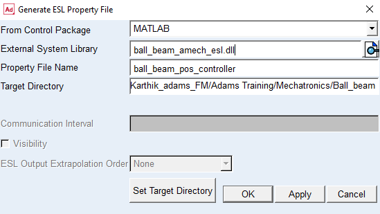
Now go back to Adams View to generate ESL property file via Mechatronics → Tools → ESL Property File …
Select the Control Package to use, as well as the .dll for Windows and .so for Linux just created in MATLAB or Easy5. Choose a name of the property file you want, as well as the location of the property file, as shown below:
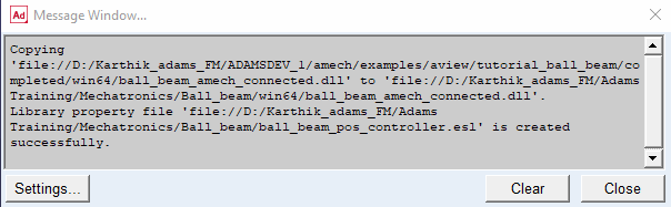
Upon successful creation of the ESL property file, you will see the following message:
The generated ESL file looks like the following.
$---------------------------------------------------------MDI_HEADER
[MDI_HEADER]
FILE_TYPE = 'esl'
FILE_VERSION = 2.0
FILE_FORMAT = 'ASCII'
HEADER_SIZE = 9
(COMMENTS)
{comment_string}
'Number of Inputs = 3, Number of Outputs = 1
Communication Interval = 1.0E-02, Visibility = 0'
$------------------------------------------------------------ROUTINE
[ROUTINE]
CONTROL_PACKAGE = 'MATLAB'
LIBRARY = 'ball_beam_amech_esl'
ROUTINE = 'ball_beam_amech_esl'
$----------------------------------------------------------PARAMETER
[PARAMETER]
d_gain1 = 1.3
d_gain2 = 0.16
i_gain1 = 0.0
i_gain2 = 0.005
p_gain1 = 1.0
p_gain2 = 0.2
adams_master_communication_interval = 0.01
adams_master_output_extrapolation_order = 0.0
$------------------------------------------------X_INITIAL_CONDITION
[X_INITIAL_CONDITION]
IC_state_1 = 0.0
IC_state_2 = 0.0
IC_state_3 = 0.0
IC_state_4 = 0.0
IC_state_5 = 0.0
IC_state_6 = 0.0
IC_state_7 = 0.0
IC_state_8 = 0.0
$-----------------------------------------------XD_INITIAL_CONDITION
[XD_INITIAL_CONDITION]
$-----------------------------------------------------SOLVER_CONTROL
[SOLVER_CONTROL]
esl_error_tolerance_scale = -1.0
Modify Control System for new ESL Property File
Select Mechatronics → Control System → Modify … to select the generated ESL property file as input for the control system.
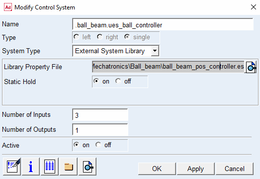
Upon selecting Apply, the library file is verified, that is, checking the number of inputs/outputs of library file vs control system defined in Adams.
Simulate Model with ESL
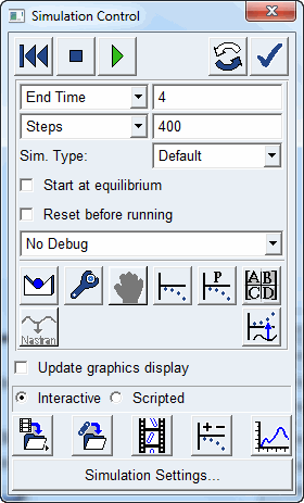
Next, perform a 4 second, 400 step simulation as follows.
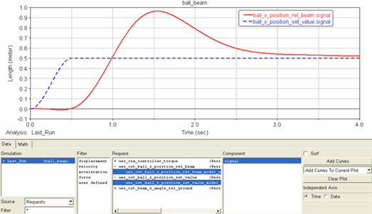
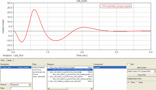
After finishing simulation, go to the Adams Post Processor to review the results. Save your results as “Original_ana”.
The following plot illustrates the actual and desired ball position with respect to time.
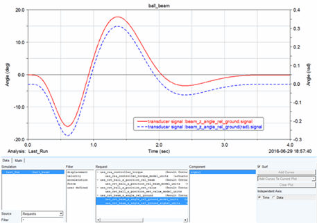
The beam angle signal can now be plotted both in signal unit (rad) and model units (deg) as shown below.
And finally the torque from the controller.
Create Disturbance and Delay and Simulate
Now you apply some disturbance and compare the results. Switch back from Adams PostProcessor to Adams View.
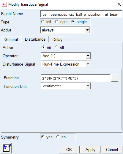
Go to the Mechatronics → Mechanical System → Transducer Signal → Modify to modify the ball_position signal by adding a disturbance signal as shown below.
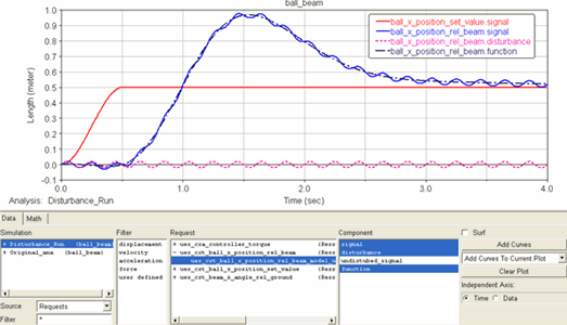
Rerun the simulation, save the result as “Disturbance_Run”, and plot the result. You can easily plot the different signal components as depicted below. You may refer to the online help to review the request definition with existence of disturbance.
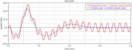
Review the disturbance effect on output torque.
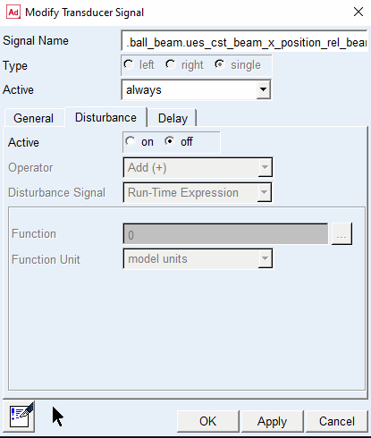
Now return to Adams View and you deactivate the disturbance by modifying the Transducer Signal shown below:
And apply a Delay of 0.03 sec
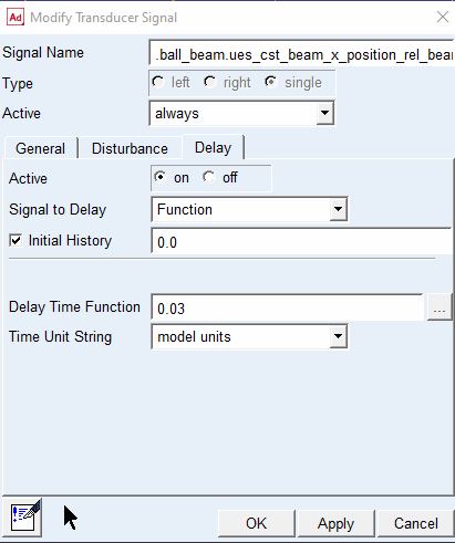
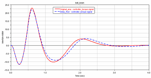
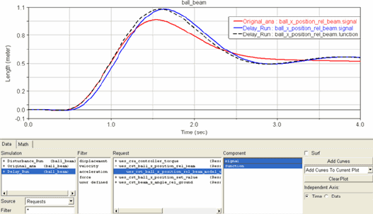
Set the solver type to C++ (which must be used to support the DELAY function) and rerun the simulation. Save the analysis result as “Delay_Run”, and plot the following requests to observe the difference in ball positions. Delay can be seen ball_x_position.signal and ball_x_position.function. For more information on the details of the delay function, see Solver guide, DELAY function.
And review the effect of applied delay on the controller torque.