Bode Plot Tutorial
This tutorial steps you through an example of how to construct bode plots when using Adams View and Adams PostProcessor together. It contains the sections:
Note: | To run this tutorial, you must use Adams PostProcessor with Adams View. You cannot use standalone Adams PostProcessr. |
About the Tutorial
We’ve provided an example command file called bode_tutorial.cmd in the install_dir\aview\examples\user_guide directory of your Adams installation directory. It contains an idealized model of a rocket and a payload.
A force with an unspecified thrust function propels the rocket, and the payload interacts with the rocket though a spring. Both the rocket body and the payload body are constrained to have a single degree of freedom (DOF) each along the x-axis. A drag force is acting on both bodies. Figure 1 shows the model.
Figure 1 Idealized Model of Rocket and Payload
About Example Model’s Input and Output
The model has a single input and a single output. The system input is a measure of the thrust, and the system output is velocity of the payload relative to ground.
The force balance equation for the rocket is:
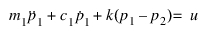
where:
■ and
and  are the positions of the rocket and payload.
and are the positions of the rocket and payload.■ and
and  are the are mass and drag coefficient for the rocket
and are the are mass and drag coefficient for the rocket■k is the connecting stiffness.
■u is the thrust.
■Dots denote time derivatives.
The force balance equation for the payload is shown below where  and
and  are mass and drag coefficients:
and are mass and drag coefficients: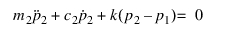
Solving the second equation for  and substituting the solution in the first equation, you will find, after some algebra, where the parameterized values denote time derivatives:
and substituting the solution in the first equation, you will find, after some algebra, where the parameterized values denote time derivatives:
Substituting the following parameter values from the example model:
■m1 = 100kg
■m2 = 10kg
■c1 = 20Ns/m
■c2 = 2Ns/m
■k = 10N/m
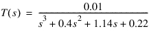
You get the following:

which yields the transfer function:
You can also introduce a change of variables:

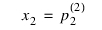
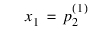
and noting that  is the output variable y, you can achieve first-order form of the differential equation:
is the output variable y, you can achieve first-order form of the differential equation: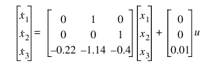
and an output equation:
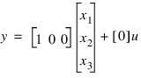
The ABCD matrices are evident in the two equations.
In the example, you will investigate the frequency response in the 0.01 Hz to 10 Hz range. You will do so using four of the seven modes of Bode plots. The remaining three modes are simple extensions of these four.
Investigating the Frequency Response
The command file bode_tutorial.cmd creates the idealized model of a rocket and payload shown in Figure 1. It defines the following elements for you:
■Rocket and payload parts.
■Connecting spring, drag, and thrust forces.
■Translational joints connecting the two parts to ground.
■Plant input element containing the Thrust_value measure that defines the thrust function used in the thrust force.
■Plant output element containing the Payload_velocity measure that defines the velocity of the payload relative to ground.
In the next sections, you’ll do the following:
■Create A, B, C, D matrices, as derived earlier, that analytically describe the system.
■Modify the measure Thrust_value so it defines a SWEEP function that applies harmonic excitation of unit amplitude and a linearly varying frequency.
■Run a simulation and generate linear state matrices, using Adams Linear.
■Generate Bode plots for each type of construction method.
You must have Adams Linear to run the portion of this tutorial that generates linear state matrices. To purchase Adams Linear, see your MSC sales representative.
Setting Up the Model
In this section, you’ll import the model, create ABCD matrices for it, and modify the Thrust_value function measure.
To set up the model:
1. Copy the file /install_dir/aview/examples/user_guide/bode_tutorial.cmd to your working directory. install_dir is the directory where the Adams software is installed. If you cannot locate the directory, see your system administrator.
Note: | By default on Windows, files in the installation directory are read-only. During installation, your system administration can choose to change the permissions so you can write to the installation directory. If this has not been done, you will need to change the permission of the above file when you copy it to your working directory. |
2. Start Adams View, and import the command file bode_tutorial.cmd.
3. Create A, B, and C data element matrices as listed below. Because D is a 1 x 1 zero matrix, you do not need to define it. As you create the matrices, name them A, B, and C, use full format, and order the matrices by row. For complete instructions on creating matrices, the Adams View online help.
■A is a 3 x 3 matrix input with the values:
0.0, 1.0, 0.0,
0.0, 0.0, 1.0,
-0.22, -1.14, -0.4
■B is a 3 x 1 matrix with the values:
0.0
0.0
0.01
■C is a 1 x 3 matrix with the values:
1.0, 0.0, 0.0
4. Create a thrust function by modifying the Thrust_value function measure to the following:
sweep(time,1.0,1.0,.001,100.0,1.0,0.01)
The thrust function defines a frequency sweep function that applies harmonic excitation of unit amplitude and a linearly varying frequency starting at 0.001 Hz at 1 second and increasing to 1 Hz at 100 seconds with a 0.01 second lead to smooth the transition. Note the parallels to a shaker table.
For complete instructions on modifying a measure, see Defining Output Using Measures in the Adams View online help.
Simulating the Model
Now you’ll simulate the model and construct linear state matrices. You can only construct linear state matrices if you have Adams Linear. If you do not have Adams Linear, you can still proceed with the rest of the tutorial.
To simulate the model and construct matrices:
1. Simulate the model for 100 seconds with 1023 output steps, for a total of 1024 (a power of two) output points.
Note: | In this example, the number of output steps is a power of two minus one. By specifying an even power minus one, the number of data points in the results is a power of two (the output steps you requested plus one for the model’s initial condition). While this is not required, we recommend you do so to obtain peak performance for Bode calculations. For more information on simulating models in Adams View, see the Adams View online help. |
2. Construct linear state matrices by linearizing the system at its state at 100 seconds if you have Adams Linear. If you do not have Adams Linear, continue to the next section.
To linearize the system:
a. From the Simulation Controls dialog box, select the Linear State Matrix tool  .
.
.b. In the dialog box that appears, enter the plant input and output. Double-click the text boxes to display the Database Navigator.
c. Select OK.
Constructing Bode Plots
You are now ready to construct Bode plots of the system for linear state matrices, ABCD matrices, transfer function coefficients, and measures.
To construct Bode plots:
1. Display the plotting window.
2. On the Plot menu, select Bode Plots.
The Bode Plot dialog box appears.
3. From the Input Format option menu, select Adams Linear State Matrices if you computed state matrices in the previous section. If you did not, continue with Step 5.
4. Enter the Linear State Matrix results object, and request a frequency range of 0.01 to 1 with 100 logarithmically spaced output points. Select Apply.
The Bode plots appear in the plotting window as shown in Figure 2. The plot shows the accumulated curves.
5. Now, from the Input Format option menu, select Adams Matrices. Browse for the A, B, and C matrices defined earlier. Leave the D text box blank and choose the same frequency sampling as in Step 4. Select Apply.
The Bode plots appear in the plotting window as shown in Figure 2. The plot shows the accumulated curves.
6. From the Input Format option menu, select Transfer Function Coefficients, and select the numerator coefficient of 0.01 and denominator coefficients of 1.0, 0.4, 1.14, and 0.22. Choose the same frequency sampling as in Steps 4 and 5. Select Apply.
The Bode plots appear in the plotting window as shown in Figure 2. The plot shows the accumulated curves.
7. Finally, from the Input Format option menu, select Time Domain Measures. Then, browse for the Thrust_value measure as input and the Payload_velocity measure as output. Because the frequency range is controlled by the time resolution of the input signals, no frequency control is available. Select OK.
The Bode plots appear in the plotting window as shown in Figure 2. The plot shows the accumulated curves.
Notice how all the four sets of curves agree in their results except for the one generated by measure data, which is slightly less accurate. You could improve the accuracy of this curve by requesting additional outputs in Step 4.
Figure 2 Bode Plot for Example Model