Modeling and Simulating Process
This explains the general mechanical system modeling and simulating process you should follow when using Adams Solver.
Process Overview
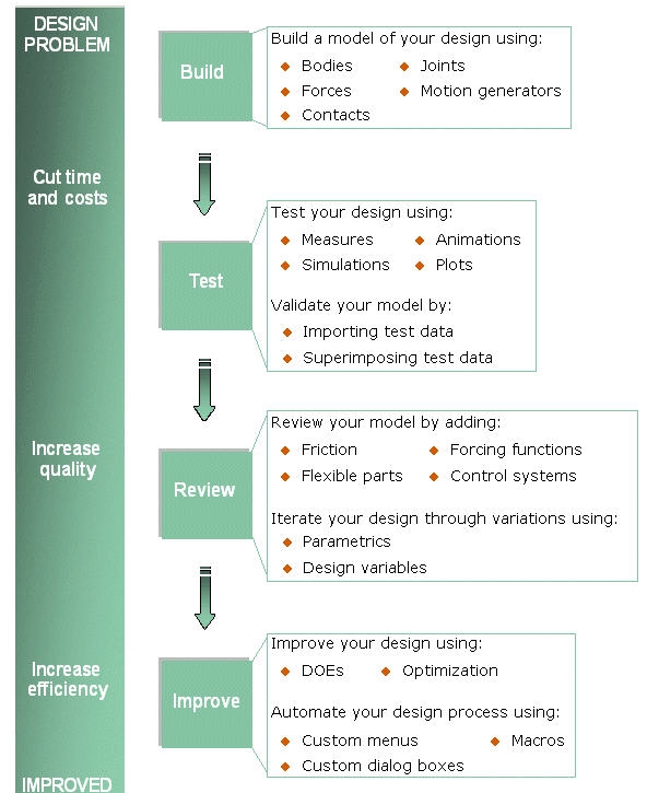
The figure below shows the steps in the modeling and simulating process. Although the steps that you perform to model and simulate a mechanical system are listed as though you build the entire model at once and then test, review, and improve it, you should build and test small elements of your model before building the entire model. For example, create a few parts, connect them together, and then run a simulation. This way you can ensure that each element works before moving on to the next step. This is referred to as the crawl-walk-run approach.
Learn more about:
■Test
Building Your Model
You define the elements of your model in a dataset. The dataset is an ASCII/text file you create using any text editor or preprocessor to enter the Adams Solver statements that describe each element of the model.
For more information about Adams Solver datasets, see Working with Adams Solver Datasets.
The build step in the process includes:
■Idealizing the mechanical system so it can be represented mathematically. This involves deciding:
■How many parts really need to be modeled.
■How to connect the parts to represent the movement of the physical system.
■Which compliant connections need to be modeled.
■Which environment forces need to be modeled.
■Selecting the units.
■Creating the basic elements. This involves:
■Creating the parts of your model.
■Adding constraints to define movement.
■Defining forces that act on your model.
■Adding system equations.
■Including requests to Adams Solver to output specific data.
Testing Your Model
After you define the model in a dataset, you can run a simulation using Adams Solver commands to verify its performance characteristics and response to a set of operating conditions.
We recommend that you simulate your model at various times during the building step. This allows you to more readily find and correct any mistakes in the model. You can also set up simulations so that they are interactive, allowing you to control and refine the simulation. During the simulation, Adams Solver solves a set of equations of motion for your model.
Reviewing the Results
As you create your model, it’s important to consider the results you want. In general, it is best to output any information you think is useful for model verification or system analysis. When you run a dynamic, kinematic, or quasi-static simulation, Adams Solver outputs data at the fixed intervals you specify. These fixed intervals are known as output time steps. When you run a static simulation, Adams Solver outputs data only once.
You can request that Adams Solver output data for displacements, velocities, accelerations, reaction forces, applied forces, user-defined variables, generic system elements, as well as system modeling element inputs and outputs. Adams Solver writes all the data you request to a request file at each output time step. Adams PostProcessor can read this file for plotting purposes. Plots are often useful for studying the specific behavior of a model. For example, if you needed to know the maximum translational loading at a joint, you could plot the translational reaction forces at the joint over the course of the entire simulation and quickly determine the maximum load. Figure 1 below shows a plot of the translational reaction forces in the translational joint between the base and the upper link of a robot arm. For more information about the wide scope of tools available in Adams PostProcessor for reviewing the response of your system, see the online help for Adams PostProcessor.
Figure 1 Plot of Translational Joint Reaction Force
Adams Solver also outputs graphical data at each output step to the graphics file. Graphical output is often useful for animating the overall behavior of the model and identifying specific problems, such as:
■Improper connectivity
■Misapplied motions or forces
■Unwanted oscillatory behavior
■Clearance problems
Figure 2 shows an animation with superimposed frames.
Figure 2 Superimposed Frames from the Animation of a Robot Arm
Improving Your Model
After you have run initial simulations to determine the basic motion of your model, you can improve and refine your model by adding more complexity to it. You can edit the dataset using more advanced statements or replace simple function expressions with subroutines. After you modify the dataset, run more simulations to verify the model.
When you have exhausted the features available in Adams Solver, you can transfer your model to Adams View to add even more complexity. For example, using Adams View, you can establish parametric relationships among modeling elements that allow you to perform design sensitivity studies to compare alternative designs. For more information about the features available in Adams View, see Adams View.
For a detailed explanation of the subroutines available in Adams Solver, see Welcome to Adams Solver Subroutines.