Understanding Adams Solver Modeling Concepts
This document contains the general modeling concepts of mechanical system simulation, and explains how Adams Solver interprets the information you provide when defining a mechanical system. It contains the sections:
Vectors
Vectors in Adams Solver are defined as quantities having magnitude and direction. They are used in mechanical system simulation to define and measure the movement of bodies, such as displacement, velocity, and acceleration. Vectors are also used to apply and measure forces in a mechanical system.
Unit vectors (where magnitude is equal to one) are most commonly used to define the direction portion of vector quantities. For example, you can use unit vectors to define the direction along which displacement, velocity, or acceleration occurs or to define the direction in which a force is applied.
Reference Frames
A reference frame specifies a reference for the calculation of velocities and accelerations in a mechanical system. Reference frames do not have any graphic representation, but are used when specifying function expressions which represent time derivatives of vector quantities. There are two types of reference frames in Adams Solver:
■Ground coordinate system (GCS) - The GCS is the single Newtonian or inertial reference that establishes absolute rest. By definition, any point attached to the GCS has zero velocity and acceleration. Such a point is fixed in absolute space.
Adams Solver expresses Newton's Laws with respect to the GCS. For many applications, you can consider the earth as a Newtonian reference frame, even though it travels in an elliptical path about the sun and is therefore accelerating, and rotates on its own axis.
■Body coordinate system (BCS) - Every rigid body has one reference frame, named the BCS.
Coordinate Systems
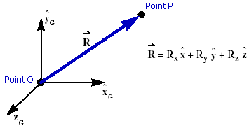
A coordinate system (CS) is essentially a measuring stick used to define kinematic and dynamic quantities. Coordinate systems usually consist of an origin and a set of three mutually-perpendicular unit vectors that specify three directions. Associated with each of these directions is a scale that permits measurement of quantities with respect to that coordinate system. You can specify all kinematic and kinetic vector quantities as projections of the vector along three mutually-perpendicular unit vectors,  ,
,  , and
, and  , as shown in the example of a Coordinate System and Vector below.
, , and , as shown in the example of a Coordinate System and Vector below.The example below illustrates a vector, R, that is defined as the displacement of point P with respect to point O. For example, R x, R y, and R z are defined as the measure numbers of R along the  ,
,  , and
, and  axes, respectively, of the global coordinate system.
, , and axes, respectively, of the global coordinate system.Example of a Coordinate System and Vector
In Adams Solver, you use coordinate systems to define:
■Location or orientation of other coordinate systems.
■Point with respect to which a body's mass moments of inertia are defined.
■Axes about which a body's mass moments of inertia are defined.
■Points at which constraints are applied.
■Axes along or about which bodies are constrained to move.
■Points to which forces are applied.
■Axes along or about which forces are applied.
You can also use coordinate systems in Adams Solver to measure:
■Translational displacement of one point with respect to another point.
■Translational velocity or acceleration of one point with respect to some reference frame.
■Angular velocity or angular acceleration of one reference frame with respect to another reference frame.
■Translational force or rotational force components acting on a body.
Adams Solver uses two types of coordinate systems, global and local, as introduced next.
Global Coordinate System
The global coordinate system (GCS) rigidly attaches to the ground reference frame or the ground body. In Adams Solver, your model has only one GCS that defines the absolute point (0,0,0) and provides a set of axes that is referenced when creating body coordinate systems (see Body Coordinate Systems).
Local Coordinate Systems
In your model, you can use local coordinate systems to identify the location and orientation of key points and axes. The origin of a local coordinate system defines its location or translational position in a mechanical system, while the axes define its orientation or rotational position.
The next sections provide information about the two types of local coordinate systems: body coordinate systems and markers.
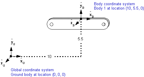
Body Coordinate Systems
A body coordinate system (BCS) is created automatically for each rigid body you define in Adams Solver. Every rigid body in your model has one and only one BCS. You specify the initial location and orientation of each BCS by providing its location and orientation with respect to the GCS. The BCS defaults to the same location and orientation as the GSC, if you do not specify a different position for it. The BCS moves with its body.
Example of Global and Body Coordinate Systems
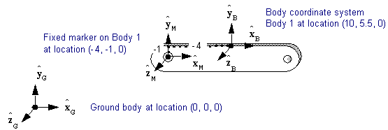
Markers
Markers are coordinate systems owned by a body. There is no limit on the number of markers you can have in your model. You use markers to define any point of interest in a mechanical system such as:
■The location of a body's center of mass.
■The reference point with respect to which you specify a rigid body's mass moments of inertia.
■A reference point for defining where you want graphical entities anchored.
■An initial location of a constraint you want to use to connect bodies together.
■A point where you want force applied to a body.
■All points where you want to measure displacement, velocity, acceleration, or force.
You can also use markers to define directions in a mechanical system such as:
■The axes about which you specify a body's mass moments of inertia.
■A direction you want to use when you specify a constrain.
■A direction you want to use when you specify a force.
■A direction you want to use when you specify graphical dimensions.
■The axes along which you want to measure displacement, velocity, acceleration, or force.
Example of Body and Marker Coordinate Systems
You have two types of markers in Adams Solver:
■Fixed markers - A fixed marker attaches to a body and moves with that body. To place a fixed marker on a body, you must specify its location and orientation with respect to the BCS.
■Floating markers - You use a floating marker to specify sites for applying certain forces or constraints to bodies. The force or constraint dictates the location and orientation of the floating marker. Therefore, you do not specify a position for a floating marker. This allows the floating marker's location and orientation to change with respect to its BCS during the simulation, as dictated by the force or constraint.
Adams Solver forces and constraints that use floating markers include the six-component force, three-component force, three-component torque, curve-to-curve constraint, and point-to-curve constraint.
Positioning Methods
You can tell Adams Solver the position of a local coordinate system by indicating its location and orientation. There is only one way to locate a local coordinate system but two ways to orient it. A local coordinate system's location is always defined the same way, regardless of the orientation method you use. In this section, the local coordinate system that you are either locating or orienting is referred to as the positioned coordinate system and the coordinate system with respect to which you are locating or orienting it as the base coordinate system. For example, if you are locating a BCS with respect to the GCS, the BCS is the positioned coordinate system and the GCS is the base coordinate system. Similarly, if you locating a marker with respect to its BCS, the marker is the positioned coordinate system and the BCS is the base coordinate system.
Note: | When you locate and orient coordinate systems, remember that the BCS is always defined with respect to the GCS and a marker is always defined with respect to the BCS of the body that owns it. |
The next sections explain the Adams Solver location and orientation positioning methods.
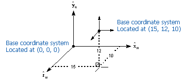
Location Method
Adams Solver uses Cartesian coordinates to define the location of the origin of the positioned coordinate system with respect to the base coordinate system. Cartesian coordinates are the distances to the point you are defining, measured from the origin and along the  ,
, , and
, and  axes of the base coordinate system. The example of the Cartesian Coordinates Location Method below shows an example of using Cartesian coordinates to define the location of a positioned coordinate system.
,, and axes of the base coordinate system. The example of the Cartesian Coordinates Location Method below shows an example of using Cartesian coordinates to define the location of a positioned coordinate system.Example of the Cartesian Coordinates Location Method
Orientation Methods
For orienting any BCS with respect to the GCS or any marker with respect to its BCS, you can use the rotation sequence method or the three-point method (also known as the direction cosines method) as explained next.
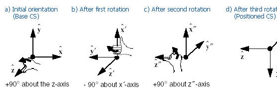
Rotation Sequence Method
The rotation sequence method used by Adams Solver to orient a local coordinate system uses rotation angles associated with a particular sequence. Although there are 24 possible rotation sequences available, Adams Solver uses only the body-fixed 3-1-3 (or z-x´-z´´) rotation sequence. The rotation angles associated with this sequence are often referred to as Euler angles. When you use the Euler angles method to orient a positioned coordinate system, you need to define the orientation of the positioned coordinate system with respect to the base coordinate system.
The example below of the Rotation Sequence Method (Body-Fixed 3-1-3 Euler Angles) shows how successive rotations of Euler angles incrementally orient the axes of the positioned frame. Initially, the positioned coordinate system has the same orientation as the base coordinate system (5a).
■The first Euler angle rotates the positioned coordinate system about its z-axis +90 degrees. This repositions the x- and y-axes (5b).
■The second Euler angle rotates the positioned coordinate system about its new x-axis (x´) -90 degrees, to reposition the new y-axis and the z-axis (5c).
■The third Euler angle rotates the positioned coordinate system about its new z-axis (z´´) +90 degrees, to reposition the new x-axis (x´´) and the second new y-axis (y´´).
Together and in sequence, these rotations define the orientation of the positioned coordinate system (5d).
The right-hand rule defines the direction of positive rotation about each axis. For example, if you look down the initial z-axis, positive rotations are counterclockwise and negative rotations are clockwise.
Example of the Rotation Sequence Method (Body-Fixed 3-1-3 Euler Angles)
Because Euler angle rotations cumulatively define the orientation, you may find it difficult to imagine orientations that involve rotations of other than 0, 45, or 90-degree increments. When orienting a coordinate system that requires a complex combination of rotations, you may find it easier to use the three-point orientation method, as described next.
Three-Point Method
You can use the three-point method to specify the orientation (in direction cosines) of the positioned coordinate system relative to the base coordinate system. When you use the three-point method to orient a positioned coordinate system, provide the following geometric data with respect to the base coordinate system:
■Cartesian coordinates of the positioned coordinate system origin (point 1). You must specify this point when using this method of orientation.
■Cartesian coordinates of a point on the primary axis of the positioned coordinate system (point 2). You can specify either the z- or x-axis as the primary axis of the positioned coordinate system. If you do not specify a primary axis, the
z-axis is used by default. When it is important to exactly specify the z-axis of the positioned coordinate system, provide the Cartesian coordinates of a point on the z-axis. When it is important to exactly specify the x-axis of the positioned coordinate system, provide the Cartesian coordinates of a point on the x-axis.
z-axis is used by default. When it is important to exactly specify the z-axis of the positioned coordinate system, provide the Cartesian coordinates of a point on the z-axis. When it is important to exactly specify the x-axis of the positioned coordinate system, provide the Cartesian coordinates of a point on the x-axis.
■Cartesian coordinates of a point that is in the x-z plane of the positioned coordinate system (point 3). Since three points in a straight line do not uniquely define a plane, you must make sure that point 3 does not lie on the line defined by points 1 and 2. If the three points are collinear, Adams Solver returns an error.
The example of the Three-Point Method below shows the points of the positioned coordinate system with respect to the base coordinate system. Point 2 in the figure specifies the z-axis of the positioned coordinate system and point 3 defines a point in the x-z plane of the positioned coordinate system. Note that in this example, point 3 is placed directly on the x-axis of the positioned coordinate system but only needs to be in the x-z plane.
By default, Adams Solver assumes that  defines the the exact location of the coordinate system origin and
  defines a point on the z-axis. Because the third point (
 by default) does not necessarily lie on an axis but happens to in this example, Adams Solver determines the vector cross product of vectors
  and
and  to form an orthogonal y-axis. Then, Adams Solver determines the vector cross product of the new y-axis and the exact axis (the z-axis by default) to produce the orientation of the remaining axis (by default, the x-axis). By calculating
  and
and  , you can verify that the third point is in the x-z plane and that the three points are not collinear.
defines the the exact location of the coordinate system origin and defines a point on the z-axis. Because the third point ( by default) does not necessarily lie on an axis but happens to in this example, Adams Solver determines the vector cross product of vectors and to form an orthogonal y-axis. Then, Adams Solver determines the vector cross product of the new y-axis and the exact axis (the z-axis by default) to produce the orientation of the remaining axis (by default, the x-axis). By calculating and , you can verify that the third point is in the x-z plane and that the three points are not collinear.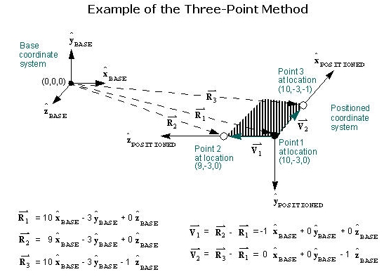
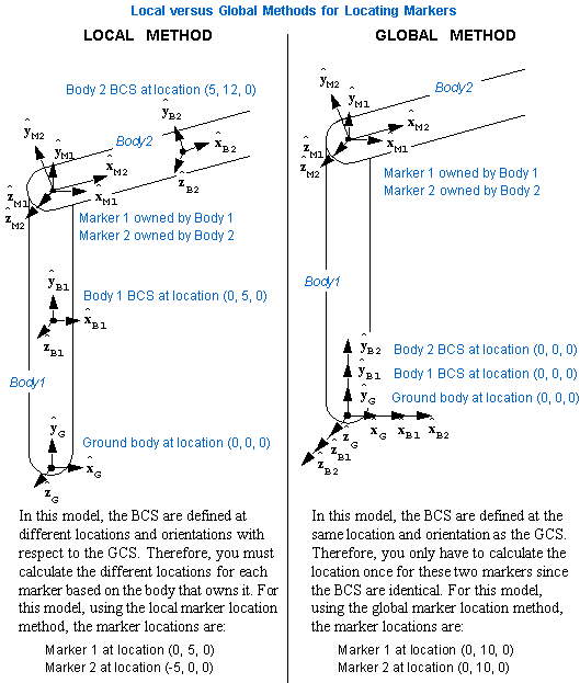
Local Versus Global Geometric Data
Regardless of the methods that you use to position the local coordinate systems, the location and orientation of every marker with respect to the GCS is the summation of both BCS and marker positioning data. This summation allows you to input points from a series of part drawings in which each drawing has its own BCS. The geometric data you input to describe the location and orientation of each BCS with respect to the GCS relates the BCS to one another.
Although the summation of the geometric data allows you to input data from part drawings with different BCS, it can complicate the process of superimposing markers in global space and assigning parallel or perpendicular orientations to their axes. Superimposing markers is sometimes necessary for defining joints (superimpose one marker on one body with a second marker on another body). For example, if you define a spherical or ball-and-socket joint, you must superimpose a marker origin at the center of the ball with a marker origin at the center of the socket. Similarly, to allow for the proper assembly of the model, certain joints require that one axis of a marker in one body remains parallel or perpendicular to a particular axis of a marker in the other body.
If two markers do not have the correct origin locations or axis orientations, Adams Solver iteratively repositions the bodies to bring the two markers to the correct position before continuing the analysis. For two markers whose positions are reasonably close to what they should be, these iterations usually do not seriously affect the solution process. For two markers whose positions are not reasonably close, Adams Solver might not be able to enforce the proper positioning during the initial phases of the simulation and will be unable to solve for the model behavior. In other cases, Adams Solver may find an initial assembly position different from the intended one, thus leading to a different solution. Consequently, when you define markers, you must carefully specify their positions and the positions of their BCS.
Not all models describe the geometry of a mechanical system as explained above. For example, in the automotive industry, it is common practice to dimension all the bodies in a single, and often large, drawing of the assembly. Because Adams Solver does not require the BCS to lie within the boundaries of the bodies to which they belong, it’s possible to superimpose all of the BCS on the GCS. When you do this, the initial marker position with respect to the BCS is the same as the marker position with respect to the GCS. Under these circumstances, the BCS positions are all zero. Because they default to zero if left unspecified, this approach reduces the amount of data that you must provide.
In addition, even though you input the markers’ positions with respect to their different BCS, all markers occupying the same position in space have identical position with respect to the GCS. In general, this approach greatly simplifies the summation process for superimposing marker positions. When using this approach, keep in mind that Adams Solver superimposes the disparate BCS on the GCS only at time zero. As the model articulates during a subsequent dynamic, kinematic, or quasi-static equilibrium analysis or settles during a subsequent static equilibrium analysis, the BCS move with their bodies with respect to the stationary GCS.
An example of local versus global data
Degrees of Freedom
Degrees of freedom dictate how a mechanical system is allowed to move. The following sections provide information on understanding and calculating degrees of freedom in your model.
Removing Degrees of Freedom
In mechanical systems, a degree of freedom (DOF) is a measure of how bodies can move relative to other bodies. Therefore, the total number of degrees of freedom of a mechanical system is the number of independent motions that characterize the model.
A freely floating rigid body in three-dimensional space is said to have six DOF. This implies that the body can exhibit motion in six independent ways: three translations and three rotations. The DOF of a mechanical system represent the minimum number of displacement coordinates needed to completely specify the system configuration. Once you know these, you can calculate any other information pertinent to the configuration as a function of these independent variables.
You can, of course, represent a mechanical system with more coordinates than there are degrees of freedom. In such an instance, the coordinates are not all independent. There must be algebraic constraint equations relating some of the coordinates. This is precisely how Adams Solver works.
For most mechanical systems, the number of degrees of freedom is constant throughout time. In some mechanical systems, the number of degrees of freedom can change as their configurations change over time.
Adams Solver allows you to specify the position of each body in the model, regardless of the degrees of freedom in the mechanical system. Different types of constraints constrain different combinations of motion, thereby removing various DOF from the model. Revolute joints, for example, constrain two degrees of rotational freedom and three degrees of translational freedom therefore allowing one degree of rotational freedom. Cylindrical joints constrain two degrees of rotational and two degrees of translational freedom, therefore allowing one rotational and one translation freedom. Rotational or translation motions, defined at joints, constrain either one rotational or translational DOF, respectively. Below tables list the number of DOF removed by Adams Solver constraints.
This joint type: | Removes number translational DOF: | Removes number rotational DOF: | Removes total number DOF: |
|---|---|---|---|
Constant velocity | 3 | 1 | 4 |
Cylindrical | 2 | 2 | 4 |
Fixed | 3 | 3 | 6 |
Hooke | 3 | 1 | 4 |
Planar | 1 | 2 | 3 |
Rack-and-pinion | 0.5* | 0.5* | 1 |
Revolute | 3 | 2 | 5 |
Screw | 0.5* | 0.5* | 1 |
Spherical | 3 | 0 | 3 |
Translational | 2 | 3 | 5 |
Universal | 3 | 1 | 4 |
* The rack-and-pinion and screw joints are shown as half translational and half rotational because they relate a translational motion to a rotational motion. They each create one constraint, but the constraint is neither purely translational nor purely rotational.
This type of joint primitive: | Removes Number translational DOF: | Removes number rotational DOF: | Removes total number of DOF: |
|---|---|---|---|
Atpoint | 3 | 0 | 3 |
Inline | 2 | 0 | 2 |
Inplane | 1 | 0 | 1 |
Orientation | 0 | 3 | 3 |
Parallel Axes | 0 | 2 | 2 |
Perpendicular | 0 | 1 | 1 |
This type of constraint | Removes number trans. DOF: | Removes number rotational DOF: | Removes number mixed translational & rotational DOF: | Removes number new generalized DOF: | Removes total number DOF: |
|---|---|---|---|---|---|
Coupler | -- | -- | 1 | -- | 1 |
Curve-to-curve | -- | -- | -- | 2 | 2 |
Gear | -- | -- | 1 | -- | 1 |
Translational motion | 1 | -- | -- | -- | 1 |
Rotational motion | -- | 1 | -- | -- | 1 |
Point-to-curve | -- | -- | -- | 2 | 2 |
User-defined constraint | -- | -- | 1 | -- | 1 |
Calculating Degrees of Freedom Using the Gruebler Equation
To determine the total number of degrees of freedom (DOF) for a mechanical system, you can use the Gruebler equation which is:
Degrees of freedom = [ 6 * (Number of movable bodies) ] - (Number of constraints)
To evaluate this equation, you would count the number of movable bodies in your model and subtract the DOF removed by the constraints and prescribed motions. Note that the body count does not include the ground body since it does not contribute any DOF. For example, the Gruebler equation for a model that contains three movable bodies, one rotational motion, three revolute joints, and one translational joint would be:
DOF = ( 6 * 3 ) - ( 1 + 5 + 5 + 5 + 5 ) = 18 - 21 = -3
From this calculation, you see that the model has -3 DOF. When the Gruebler equation yields a DOF count less than zero, it indicates that the model definitely has one or more constraints that are redundant.
If you use the same model and replace one of the revolute joints with a spherical joint and another revolute joint with a cylindrical joint, the Gruebler equation would then be:
DOF = ( 6 * 3 ) - ( 1 + 5 + 3 + 4 + 5 ) = 18 - 18 = 0
This equation now indicates that there are zero DOF in the model. When the Gruebler equation is greater than or equal to zero, you cannot be positive that the mechanical system does not contain constraints that are redundant.
The Gruebler equation offers a good way to understand how the model is built, but to see if there are redundant constraints or not, it is best to let Adams Solver perform an analysis. You will receive a message from Adams Solver if the model contains redundant constraints. However, you do not know how many or which ones Adams Solver sees as the redundant constraints. For information on how Adams Solver handles models with redundant constraints, see Checking for Redundant Constraints below.
Checking for Redundant Constraints
You can construct a legal and well-defined model where one set of joints constrain the model in exactly the same way as another set of joints. In mathematical terms, you can state that the equations of constraint of both sets of joints are redundant with each other.
An Adams Solver model is a mathematical idealization of a physical mechanical system. For this reason, your model can contain redundant constraints even if you define your model with the same number and types of joints as the physical mechanical system.
An example of a mechanical system with redundant constraints is a door supported by two hinges. In a real door, minor violations of the hinge collinearity do not prevent the door from operating because of body deformity and joint-play in the hinges. In the mathematical model, where the bodies are rigid and joints do not permit any play, the two hinges are redundant but consistent when the axes of the two hinges are aligned. If, however, the axes are not aligned, the door cannot move without breaking one of the hinges. In this case, the two hinges are inconsistent and half of their constraints are redundant.
Adams Solver does not tolerate redundant constraints whether they are consistent or inconsistent. When encountered, Adams Solver subjectively determines which constraints are redundant, deletes them from the set of equations, and provides a set of results that characterize the motion and forces in the model. Note that other solutions can also be physically realistic. Systems with redundant constraints do not have a unique solution.
According to the Gruebler equation, an Adams Solver model with fewer than zero DOF is overconstrained. Adams Solver can solve an overconstrained model only if the redundant constraints are consistent. Redundant constraints are consistent if a solution satisfying the set of independent constraint equations also satisfies the set of dependent or redundant constraint equations.
In the case of the door with two hinges, Adams Solver ignores five of the constraint equations. You, unfortunately, do not know which equations are removed. If you assume that Adams Solver ignores all of the equations corresponding to one of the hinges, that means that all the reaction forces are concentrated at the other hinge in the Adams Solver solution. Adams Solver subjectively sets the reaction forces to zero at the redundant hinge. However, as long as distribution of reaction forces maintains a constancy of the net reaction force and torque, it also provides a correct solution.
Adams Solver does not always check joint initial conditions when it does overconstraint checking. If you apply a motion on one joint and initial conditions on another joint, check to make sure that they are not redundant because Adams Solver does not check them. As a general rule, you should not specify more initial conditions than the model has degrees of freedom.
For a model with redundant constraints, constraints that are initially consistent can become inconsistent as the model articulates over time. Adams Solver stops execution as soon as the redundant constraints become inconsistent. Therefore, you should not intentionally input redundant constraints in your model. For example, consider a planetary gear system with redundant constraints. Slight misalignment errors can accumulate over time, eventually resulting in a failure of the consistency check. If this occurs, manually remove the redundant constraints or replace them with flexible connections.
If you have redundant constraints in your model, try replacing joints with joint primitives or with approximately equivalent flexible connections. By reviewing the messages saved in the message file after Adams Solver tries to solves your model, you can find out how many and which redundant constraints are being removed.
Force Direction and Application
You can define any force vector in terms of its magnitude and direction. The following sections explain how Adams Solver directs and applies the different forces available.
Single-Component Forces
You can use two types of single-component forces in Adams Solver:
Action-Only, Single-Component Forces
An action-only, single-component force is an external force or torque applied to a single body in a model that acts along a specified fixed axis. As you know from Newton’s third law, however, in nature there is no such thing as an action-only force (that is, one with no reaction). Therefore, the body reacting to the action-only force in Adams Solver is automatically defined as ground and shows no visible effect in your model.
Note: | You may find the action-reaction, multi-component forces more intuitive to use than the action-only, single-component force. If you want to apply force to only one body, you can use the action-reaction, multi-component forces and specify the reaction marker on ground. |
You can apply either a translational or rotational action-only, single-component force to a body in your model. Note that a rotational force is a pure torque in Adams Solver. For both translational and rotational action-only, single-component forces, you provide Adams Solver with two markers: action and direction. The action marker declares the point of application for the force.
For a rotational force, or pure torque, the location of the action marker is irrelevant; only the body to which it belongs is important. The z-axis of the direction marker specifies the direction of the force. Adams Solver evaluates the signed magnitude and applies it to the action marker.
If the force is positive and translational (Figure 3), it acts in the positive direction along the z-axis of the direction marker. If the force is positive and rotational (Figure 4), it acts in the positive direction about the z-axis of the direction marker. The right-hand rule defines the positive direction.
Figure 3 Translational, Action-Only, Single-Component Force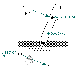
Figure 4 Rotational, Action-Only, Single-Component Torque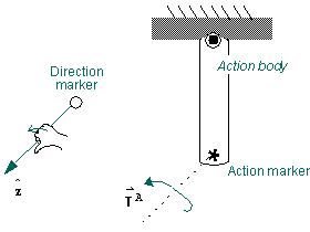
Action-Reaction, Single-Component Forces
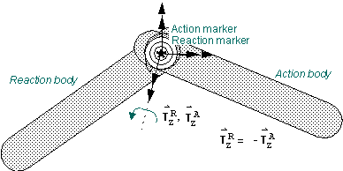
An action-reaction force is a force applied to one body producing a reaction force on a second body that is equal and opposite to the action force on the first body. You can apply either a translational or rotational (torque) action-reaction, single-component force to your model.
■For translational, action-reaction, single-component forces (Figure 5), you provide Adams Solver with two fixed markers: action and reaction. These markers specify the points of force application and the line along which the instantaneous forces act, therefore no direction marker is needed. If the force applied to the action marker is positive, the action marker is pushed away from the reaction marker. If the force applied to the action marker is negative, the action marker is pulled towards the reaction marker.
■For rotational, action-reaction, single-component torques (Figure 6), you provide Adams Solver with two fixed markers: action and reaction. These markers only specify the body affected by the torque not a location on the body itself, because pure torques are independent of location. The z-axis of the reaction marker specifies the axis about which the torque is applied. If the torque is positive, the action marker tends to move counter-clockwise to the reaction marker. If the torque is negative, the action marker tends to move clockwise to the reaction marker.
Figure 5 Translational, Action-Reaction, Single-Component Force
Figure 6 Rotational, Action-Reaction, Single-Component Torque
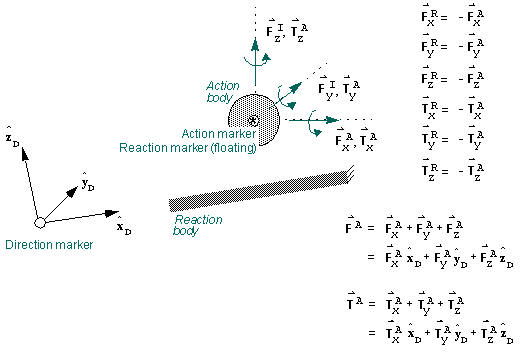
Multi-Component Forces
Adams Solver also allows you to define multi-component translational and rotational force vectors. For each of the multi-component forces, you provide Adams Solver with two fixed and one floating marker: action (fixed), reaction (floating), and direction (fixed). The action and reaction markers always remain coincident. The axes of the direction marker define the directions of the vector components. You specify the x, y, z measure numbers of the force components to define them with respect to the direction marker axes.
If a vector component is positive and translational (Figure 7), it acts in the positive direction along the corresponding axis of the direction marker. If a vector component is positive and rotational (Figure 8), it acts in the positive direction about the corresponding axis of the direction marker according to the right-hand rule. You should specify all of the components of each multi-component force to be applied to the action marker, even if some are zero. Equal and opposite forces are automatically applied to the reaction (floating) marker.
Figure 7 Three-Component, Action-Reaction Force 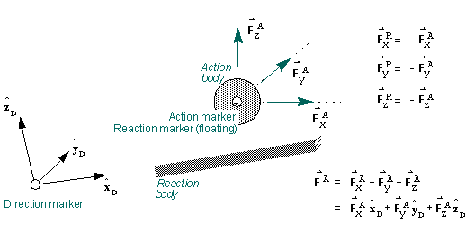
Figure 8 Three-Component, Action-Reaction Torque 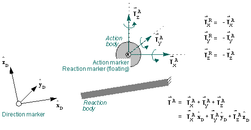
Figure 9 Six-Component, Action-Reaction Force/Torque