DELAY

Adams Basic Package > Adams Solver > Welcome to the C++ Version of Adams Solver > C++ Functions > DELAY

DELAY

The DELAY function returns the value of an expression at a delayed time.

The DELAY function is useful to define Delay Differential Equations (DDE) or Delay Differential-Algebraic Equations (DDAE) of the retarded type (when delays are positive). Neither DDE nor DDAE of the advance type (negative delays) are supported.

The DELAY function can be used in MOTION and GCON definitions (possibly involving neutral type of DDE or DDAE).

During linearization the DELAY function is approximated by a first order polynomial equivalent to an order 1 Padé approximant.

The user does not require to specify a buffer size. Adams Solver (C++) will manage a variable-size buffer automatically.

Format

DELAY (e_delayed, e_delay, e_history [, id])

Arguments

e_delayed	Adams expression to be delayed. The expression may be time and/or state dependent. The expression may be explicitly defined or it may be computed by the solver during the simulation. See Limitations section below.
e_delay	Adams expression defining the magnitude of the delay. The delay can be constant or state dependent. The magnitude of the delay must be positive. Negative values will be taken as zero.
e_history	Initial history of the expression; the history must provide for the values of 'e_delayed' for the values of time less than zero (t<0). The history must be a function of TIME or a constant.
id	The identifier of an array of type IC containing the order of interpolation, a jump threshold, an angle threshold, and a refinement parameter.

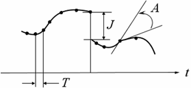
The delayed expression can have jumps and derivative discontinuities. If the signal has jumps, a jump threshold J (see Figure below) can be specified. The default jump threshold is 0.5. If the signal has corners, an angle corner threshold A (see Figure below) can be specified. The default angle corner threshold is π/8.

The default interpolation order is 6. In cases in which the delayed expression changes abruptly, a lower integration order may be required. If the interpolation order is equal to 1, the corner and jump detection are disabled.

By default the refinement parameter R is 200. The value of R controls the separation T (see Figure below) between points used by the interpolator. Only points such that

are stored in the history of the expression. In the above expression, t is the current time, tl is the last point in the stored history, and τ is the current value of the delay. The bigger the value of R, the more integration points are stored in the history of the delayed expression. The value τ /R can be seen as a lower bound for the separation between points in the delayed expression history. For delays smaller than the current integration step, R is ignored and all integration points are recorded.

Limitations

The DELAY function may be used in any force equation, constraint equation, variable equation, or a differential equation. Given that Adams Solver (C++) requires to compute time derivatives of the delayed expression, the delayed expression shall not be an acceleration expression. However, a workaround consists of wrapping the delayed expression using the AO function. See Example 4 below.

Example 1

Here we solve a simple DDE system. The equations below define a typical DDE system with a state-dependent delay expression:

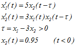
The expression to delay (e_delayed) is x2, the delay expression (e_delay) is τ, and the history (e_history) is the constant expression 0.95.

This system could be modeled in Adams as follows:

DIF/1,   FU=5*DELAY(DIF(2), DIF(1)-3*DIF(2), 0.95)) 

DIF/2,   FU=3*DIF(1)*DELAY(DIF(2), DIF(1)-3*DIF(2), 0.95)

VARIABLE/1, FU=DELAY(DIF(2), DIF(1)-3*DIF(2), 0.95)

DIF/1,      FU=5*VARVAL(1) 

DIF/2,      FU=3*DIF(1)*VARVAL(1)

Example 2

A simple mass-spring-damper system.

Figure below shows a MATLAB model to study the dynamics of a simple mass-spring-damper system governed by the following equation:

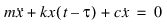
where the delay τ is given by the following expression:

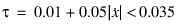
and zero initial history ( x(t)=0 for t<0 ) and

. System properties are m=1, k=30 and c=2.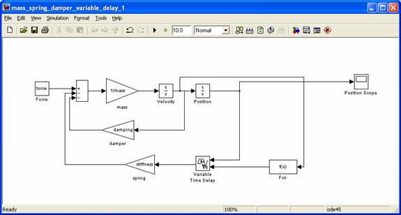

The corresponding Adams model is the following:

Simple spring-damper system
! Varying delay equal to 0.01+abs(vz(3))*0.05 < 0.035
! M=1, K=30, C=2
!
units/system=mks
!
part/1, ground
marker/1
marker/2, floating
!
part/2, mass=1, ip=1,1,1, cm=3, vz=1
marker/3
!
var/2, fun=0.01+abs(vz(3))*0.05
var/3, fun=if(varval(2)-0.035:varval(2),varval(2),0.035)
var/1, fun=-30*delay(dz(3),varval(3), 0)-2*vz(3)
!
joint/1, trans, i=1, j=3
!
vforce/1, i=3, j=2, rm=1, fx=0\ fy=0\ fz=varval(1)
!
results/formatted, xrf
end 

A discontinuous signal.

This example sets the delay to 1, the initial history to 0 and the optional array id is 77.

var/1, fun=delay(dz(3),1, 0, 77) 

!

Array/77, type=ic, size=4, numbers= 

,6   !  Order of interpolator 

,0.3 !  Jump threshold 

,0.3 !  Angle corner threshold (rads) 

,40  !  Refinement parameter R 

!

Example 3

This example illustrates the potential problem of not having smooth data fed into the history of the DELAY object. This example consists of a model that has no dynamic states; it simply defines a set of variables as follows:

Example of DELAY function

!

!                            adams_view_name='ground'

PART/1

, GROUND

!

!                      adams_view_name='reference_harmonic'

VARIABLE/1

, FUNCTION = sin(25*time)

!

!                          adams_view_name='delay_test'

VARIABLE/2

, FUNCTION = delay(varval(1), 0.5*time+0.01, 0)

!

!                           adams_view_name='feedback'

VARIABLE/3

, FUNCTION = step(time,0,0,0.05,sin(time*25))+delay(varval(3),2*PI/25,0)

!

RESULTS/XRF

!

END

We run this model for 2.0 seconds using 200 output steps and 20 output steps respectively:

sim/kin, end=2, step=200

stop

and

sim/kin, end=2, step=20

stop

The results are presented in the figure below.

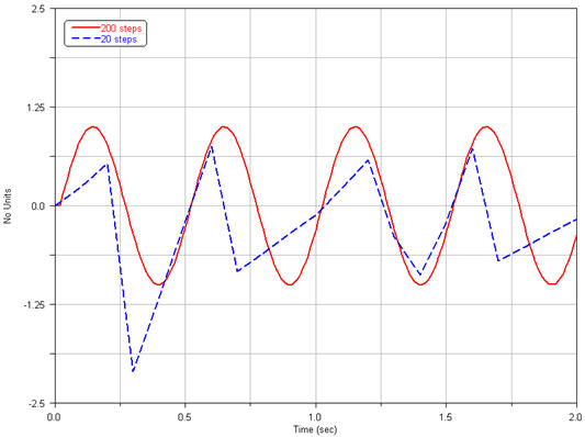
Notice the poor solution for the case of only 20 steps. The reason is that the integrator took large steps feeding a history with data that can not be properly interpreted by the interpolation algorithm used by the DELAY object.

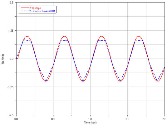
In order to remedy this behavior, one option is to specify the HMAX option of the kinematic command as follows:

kinematics/hmax=0.01

sim/kin, end=2, step=20

stop

The new solution is presented in figure below.

Example 4

This example shows the case of a function of time X(t) that depends on an acceleration. The delay value is

and the delay X(t-

) may be defined as follows. Assuming X(t) is defined in VARIABLE/2 and the delay

is defined by VARIABLE/3 we have:

VARIABLE/2, FUNCTION=SIN(TIME)*ACCX(8) ! Function X(t)

VARIABLE/3, FUNCTION=0.5 ! The delay

Then the delayed expression (VARIABLE/4) is:

VARIABLE/4, FUNCTION=DELAY(AO(VARVAL(2)), VARVAL(3), 0)

Here we assumed the initial history is zero. Notice we use the AO function to wrap the expression to be delayed.

Caution:

The DELAY function uses an internal buffer, that holds the history of the expression 'e-delayed'. This history is fed by the integrator. The number of steps or the HMAX option in the INTEGRATOR provide smooth data as shown in Example 3 above.

See other Miscellaneous Adams intrinsic functions available.