DEBUG
The DEBUG command redefines and/or lists the data for a DEBUG statement. See the DEBUG statement for more information.
Format
Click the argument for a description
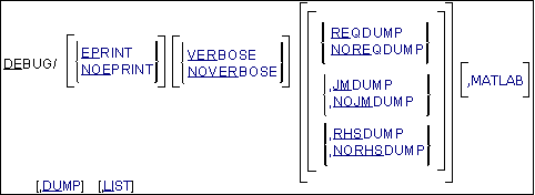
Arguments
DUMP | Writes the internal representation of a dataset in the Tabular Output File after Adams Solver reads and checks the input. This facility essentially maps the equations and variables in the system and provides their numeric codes. Default: Off |
EPRINT | Prints a block of information for each kinematic, static, or dynamic step. This information helps you monitor the simulation process and to locate the source of the error if there is a problem. Each step consists of two phases: 1) a forward step in time (the predictor for dynamics) and 2) the solution of the equations of motion (the corrector for dynamics). For the first phase, Adams Solver prints out the following information: ■The step number. This is a running count of the number of steps taken and can be used as a measure of how hard Adams Solver is working. ■The order of the predictor for dynamics. This corresponds to the order of the polynomial Adams Solver uses to predict the solution at the end of the integration step. ■The value of time at the beginning of the step. ■The size of the step. For the second phase, Adams Solver prints out the cumulative number of iterations and a table of information about the iterations. The cumulative number of iterations is a running count of the iterations needed to solve the equations of motion and can be used as a measure of how many computations Adams Solver is performing. The table contains information about the maximum equation error and maximum variable change for each iteration. For each iteration, Adams Solver prints out the following information: ■The iteration number. This is one at the beginning of each step and increments by one until Adams Solver converges to a solution or exceeds the maximum allowable number of iterations. ■The largest (in absolute value) equation residual. Each equation should have an error value close to zero. This number is an indicator of how far Adams Solver is from a solution. This number should decrease after every iteration. ■The dataset element associated with the largest equation residual error. ■The equation that has the largest equation residual error for the above dataset element. ■The absolute value of the largest change in a variable. The final iteration should not need to change variables very much. This number is an indicator of how far Adams Solver needs to change variables to approach a solution. This number should decrease after every iteration. ■The dataset element associated with the absolute value of the largest change in a variable. ■The variable with the largest change for the above dataset element. ■If Adams Solver has updated the Jacobian, YES appears under the new Jacobian header. Default: NOEPRINT |
JMDUMP | Dumps the Jacobian matrix at each iteration. The Jacobian is dumped in the working directory in the file with extension *.jac and root name equal to the one of the message file. Default: NOJMDUMP |
LIST | Lists the current values of the data in the DEBUG statement. |
NOEPRINT | Suppresses the printing of three numbers at each integration step and five numbers at each corrector iteration during an integration. Default: NOEPRINT |
NOJMDUMP | Disables the dumping of the Jacobian matrix at each iteration. Default: NOJMDUMP |
NOREQDUMP | Disables the dumping of REQUEST and MREQUEST statement output at each iteration. Default: NOREQDUMP |
NORHSDUMP | Disables the dumping of the YY array (state vector), the RHS array (error terms), and the DELTA array (increment to state vector) at each iteration. Default: NORHSDUMP |
NOVERBOSE | Deactivates the output of explanations and possible remedies and the output of the names of subroutines from which Adams Solver sends diagnostics. Default: NOVERBOSE |
REQDUMP | Enables the dumping of the REQUEST and the MREQUEST statement output at each iteration. Default: NOREQDUMP |
RHSDUMP | Dumps the values of the right-hand-side vector and states in the solution of each AX=b linear problem. The states and right-hand-side are dumped in the working directory in the file with extension *.rhs and root name equal to the one of the message file. Default: NORHSDUMP |
VERBOSE | Outputs to the screen such additional information as the name of the subroutine from which Adams Solver sends each diagnostic, explanations, and possible remedies (when available). If you do not include the VERBOSE argument, Adams Solver outputs to the screen only basic error messages. Whether or not you include the VERBOSE argument, Adams Solver outputs VERBOSE information to the Message File. Default: NOVERBOSE |
MATLAB | When specified in conjunction with the RHSDUMP or JMDUMP flags it changes the output format to be such that the debug information can be easily imported into Matlab. Importing for example the Jacobian matrix in Matlab can be useful for purposes such as computing the condition number of the Jacobian, its norm and so on. |
Extended Definition
Of all the arguments in the DEBUG command, EPRINT is perhaps the most useful. This section explains the EPRINT argument in detail.
The kinematic, dynamic, and quasi-static analyses in Adams Solver involve the solution of the governing equations of motion. Static analysis is the solution of the equilibrium and the initial conditions analysis solves the assembly equations at a particular point in time.
The equations to be solved, for all these analyses, are non-linear algebraic or differential-algebraic equations. The solution of these equations is an iterative process. The EPRINT argument enables Adams Solver to write out the information pertaining to the solution process in a succinct and understandable format. All analyses that march through time consist of two distinct phases: predictor phase and corrector phase.
Predictor Phase
In order to proceed efficiently from one time to the next, Adams Solver uses a predictor. The predictor is simply a means of estimating the values of the system state by looking at the past values of the state and extrapolating the data based on a simple curve fitting algorithm.
Consider a series of values yi defined at discrete times ti
where i=1...n. A simple first order predictor that may be used to predict the value yn+1 at tn+1 is: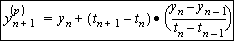
where superscript p implies a predicted value. This is shown graphically in Figure 1.
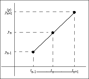
Figure 1 First Order Predictor
You can easily surmise from Figure 1, a first order predictor simply consists of connecting the points yn-1 and yn with a straight line and extending it to time tn+1.
A second order predictor, similarly, can be thought of as constructing a parabola between the points (tn-2, yn-2), (tn-1, yn-1) and (tn, yn) and extending the parabola to time tn+1. The predicted value of y at tn+1 is the intersection of the vertical line t=tn+1 with this parabola. Predictors are typically polynomials (linear, quadratic, cubic, etc.) and the order of the polynomial is frequently called the order of the solution method.
For kinematic analyses, Adams Solver employs a first or second order predictor. For quasi-statics, a first order predictor is used. For dynamic analyses much higher order predictors are used. The BDF methods (GSTIFF and WSTIFF) use up to six order predictors. ABAM on the other hand can use up to a 12th order predictor. Sophisticated numerical analysis is employed to determine the most appropriate order of prediction to use at any given step.
Furthermore, sophisticated curve fitting methods like Newton-Divided Difference tables are usually employed to efficiently predict the system state. Figure 2 shows the format of the output produced by the EPRINT argument and explains the data pertinent to the predictor phase of a dynamic analysis step.
The predictor polynomials used for the dynamic analyses interpolate previous values and the slope of the variable at the current time to estimate the solution at the next time. Therefore, in Figure 5, a second order polynomial that fits the solution at times t4 and t5 and the slope of the solution at time t5 is used to predict the value of the solution at time t6.
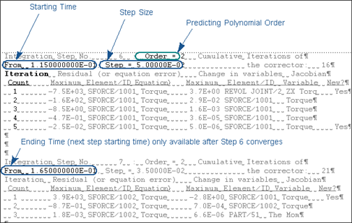
Figure 2 A Successful Integration Step
Corrector Phase
Since all predictors simply look at past values to estimate the solution at the next time, the predicted values almost never satisfy the governing equations. They simply constitute a good initial guess for the solution. The refining of the predicted solution to one that satisfies the governing equations is called the correction. Since the governing equations are usually non-linear, an iterative scheme like Newton-Raphson iterations are used.
This methodology is explained for the simplest case of one non-linear algebraic equation in one variable. Let f(x) be a smooth function of a single variable x. Given an initial guess x=x0, a solution x=xc that satisfies f(x)=0 is desired for this simple example. The Newton-Raphson iterations may be expressed as:
for i=0 ... max_no_iterations.  is a small user-defined number that specifies the convergence criterion.
is a small user-defined number that specifies the convergence criterion. 1. Evaluate ri = f(xi)
2. If || err(xi) || <  return xi as the solution
return xi as the solutionwhere err(xi) is the error measure being maintained during Newton Raphson iterations
3. Evaluate 
4. Calculate 
5. Set 
6. Set i = i+1 and go to Step 1.
The quantity ri is frequently called the residual and is a measure of the accuracy of the solution. The quantity Ji is the partial derivative of f with respect to x, evaluated at x=xi and is commonly known as the Jacobian. The graph on the left side of Figure 3 illustrates the Newton-Raphson iterations for the one-dimensional example discussed above.
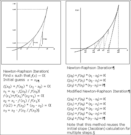
Figure 3 The Newton-Raphson Algorithm for a Single Nonlinear Equation
J0 is the slope of the curve f(x) at x=x0. Through simple trigonometry it can be seen that x0-x1 = r0/J0 (i.e., x1 = x0 - r0/J0).
Similarly,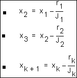
The corrector in Adams Solver involves the solution of many variables simultaneously. The algorithm for one dimension is easily extended to n dimensions as follows:
Let x = {x1, x2,... xn} be a set of n variables and f = {f1(x), f2(x),... fn(x)} be a set of n non-linear equations in the variables x.
Define:
J =  ,
,
, where i=1,...,n and j=1,...,n. Then the Newton-Raphson iterations for the n-dimensional case becomes: given an initial guess x = x0 = {x01, x02,... x0n} for i=0,...,max_no_interations.  is a small user-defined number that specifies the convergence criterion.
is a small user-defined number that specifies the convergence criterion. 1. Evaluate ri = f(xi)
2. If || ri || < return x = xi as the solution
return x = xi as the solution 3. Calculate , where j=1,...,n and k=1,...,n
, where j=1,...,n and k=1,...,n 4. Evaluate
5. Set ,
,
, 6. Set i = i+1 and go to Step 1.
For the n-dimensional case, evaluating the Jacobian Ji and its inverse at each iteration can be quite expensive and is the most expensive part of the iteration process. In order to decrease the computational overhead, the Jacobian Ji is not evaluated at each iteration. It is only updated periodically. This technique can dramatically increase the overall speed of the corrector iterations and is termed Modified Newton-Raphson iterations.
The graph on the right side of Figure 3 demonstrates the use of the Modified Newton-Raphson iterations to solve the one-dimensional problem f(x)=0. In this example, the initial Jacobian f’(x0) is re-used for the first 4 corrections before it is re-evaluated for iteration 5. The data are shown in Figure 4 for the modified Newton-Raphson iterations in a dynamic analysis. The numbers on the left are the values of the maximum residuals at each iteration. The maximum corrections are on the right. In practice, the convergence rate of the iterations is used to determine whether a Jacobian evaluation is to be performed or not.
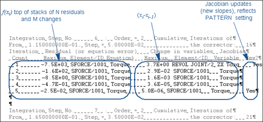
Figure 4 The Modified Newton-Raphson Algorithm for a System of Non-linear Equations
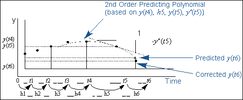
Figure 5 Predictor Polynomial and Corrected Value
The DEBUG/EPRINT option generates a table of data on the action of Adams Solver for each of the iterative algorithms in the various analyses. The iterative algorithm, or corrector, is used to evaluate the variables governed by the system of non-linear equations. Table 1 contains the DEBUG/EPRINT information for the variables associated with the mass-bearing elements (parts, point masses, and flexible bodies) and for the corresponding equations. A combination of several equations is needed to define each joint and joint primitive. Table 2 includes the variables for the various joint constraints and the corresponding equations.
Adams Solver uses a combination of equations to represent the different types of forces. While certain equations are specific to a particular force, others are generic to all types. The combination of variables and corresponding equations for the forces are included in Table 3. The DEBUG/EPRINT information for the variables and corresponding equations that define the Adams system elements is contained in Table 4. Finally, Table 5 includes the information on the variables and equations for the remaining miscellaneous elements in an Adams system.
Table 1 Mass Bearing Elements Debug Descriptions
EQUATIONS | VARIABLES | |||
|---|---|---|---|---|
Element type: | Code: | Explanation: | Code: | Explanation: |
Parts |  | Translational force, x-direction, GCS |  | Translational coordinate, x-direction, GCS |
 | Translational force, y-direction, GCS |  | Translational coordinate, y-direction, GCS | |
 | Translational force, z-direction, GCS |  | Translational coordinate, z-direction, GCS | |
 | Algebraic equation for the  component of the angular momentum component of the angular momentum |  | Rotational rate, first component, 3-1-3 Euler angles, GCS | |
 | Algebraic equation for the  component of the angular momentum component of the angular momentum |  | Rotational rate, second component, 3-1-3 Euler angles, GCS | |
 | Algebraic equation for the  component of the angular momentum component of the angular momentum |  | Rotational rate, third component, 3-1-3 Euler angles, GCS | |
 | Torque, the  component component |  |  component of the angular momentum component of the angular momentum | |
 | Torque, the  component component |  |  component of the angular momentum component of the angular momentum | |
 | Torque, the  component component |  |  component of the angular momentum component of the angular momentum | |
vx | Velocity equation, x-coordinate, GCS | x | Translational coordinate, x-direction, GCS | |
vy | Velocity equation, y-coordinate, GCS | y | Translational coordinate, y-direction, GCS | |
vz | Velocity equation, z-coordinate, GCS | z | Translational coordinate, z-direction, GCS | |
 | Equation for the time-derivative of the  coordinate coordinate |  | Rotational coordinate, first component, 3-1-3 Euler angles, GCS | |
 | Equation for the time-derivative of the  coordinate coordinate |  | Rotational coordinate, second component, 3‑1-3 Euler angles, GCS | |
 | Equation for the time-derivative of the  coordinate coordinate |  | Rotational coordinate, third component, 3‑1‑3 Euler angles, GCS | |
Flexible Bodies |  | Translational force, x-direction, GCS |  | Translational coordinate, x-direction, GCS |
 | Translational force, y-direction, GCS |  | Translational coordinate, y-direction, GCS | |
 | Translational force, z-direction, GCS |  | Translational coordinate, z-direction, GCS | |
 | First of three equations of motion for torque |  | Time-derivative of the  coordinate coordinate | |
 | Second of three equations of motion for torque |  | Time-derivative of the  coordinate coordinate | |
 | Third of three equations of motion for torque |  | Time-derivative of the  coordinate coordinate | |
 | Inertial equations for modal coordinates for 1  j j  number of flexible modes number of flexible modes |  | Time-derivatives of modal coordinates for 1  j j  number of flexible modes number of flexible modes | |
vx | Velocity equation, x-coordinate, GCS | x | Translational coordinate, x-direction, GCS | |
vy | Velocity equation, y-coordinate, GCS | y | Translational coordinate, y-direction, GCS | |
vz | Velocity equation, z-coordinate, GCS | z | Translational coordinate, z-direction, GCS | |
 | Equation for the time-derivative of the  coordinate coordinate |  | Rotational coordinate, first component, 3-1-3 Euler angles, GCS | |
 | Equation for the time-derivative of the  coordinate coordinate |  | Rotational coordinate, second component, 3‑1-3 Euler angles, GCS | |
 | Equation for the time-derivative of the  coordinate coordinate |  | Rotational coordinate, third component, 3‑1‑3 Euler angles, GCS | |
 | Equation for the time-derivatives of modal coordinates for 1  j j  number of flexible modes number of flexible modes |  | Modal coordinates for 1  j j  number of flexible modes number of flexible modes | |
Point Masses |  | Translational force, x-direction, GCS |  | Translational velocity, x-direction, GCS |
 | Translational force, y-direction, GCS |  | Translational velocity, y-direction, GCS | |
 | Translational force, z-direction, GCS |  | Translational velocity, z-direction, GCS | |
Table 2 Joint and Joint Primitive Debug Descriptions
EQUATIONS | VARIABLES | ||||
|---|---|---|---|---|---|
Element type: | Code: | Explanation: | Code: | Explanation: | Notes: |
Joint Initial Condition, | x | At Point Constraint (x) xi − xj = 0 | Reaction Force (x) | 1 | |
Translational | y | At Point Constraint (y) yi − yj = 0 | y Force | Reaction Force (y) | 1 |
z | At Point Constraint (z) zi − zj = 0 | z Force | Reaction Force (z) | 1 | |
Joint Initial Condition, | xi • yj | Angular Constraint (xi, yj) xi • yj = 0 | xy Torque | Reaction Torque (xi, yj) | 2 |
Rotational | zi • xj | Angular Constraint (zi, xj) zi • xj = 0 | zx Torque | Reaction Torque (zi, xj) | 2 |
zi • yj | Angular Constraint (zi, yj) zi • yj = 0 | zy Torque | Reaction Torque (zi, yj) | 2 | |
Cylindrical Joint | zi • xj | Angular Constraint (zi, xj) zi • xj = 0 | zx Torque | Reaction Torque (zi, xj) | 2 |
zi • yj | Angular Constraint (zi, yj) zi • yj = 0 | zy Torque | Reaction Torque (zi, yj) | 2 | |
s • xj | Sliding Constraint (s, xj) s • xj = 0 | sx Force | Reaction Force (s, xj) | 3 | |
s • yj | Sliding Constraint(s, yj) s • yj = 0 | sy Force | Reaction Force (s, yj) | 3 | |
Convel Joint | x | At Point Constraint (x) xi − xj = 0 | x Force | Reaction Force (x) | 2 |
y | At Point Constraint (y) yi − yj = 0 | y Force | Reaction Force (y) | 2 | |
z | At Point Constraint (z) zi − zj = 0 | z Force | Reaction Force (z) | 2 | |
xi • yj | Angular Constraint (xi, yj) xi • yj = 0 | xy Torque | Reaction Torque (xi, yj) | 3 | |
Fixed Joint | x | At Point Constraint (x) xi − xj = 0 | x Force | Reaction Force (x) | 1 |
y | At Point Constraint(y) yi − yj = 0 | y Force | Reaction Force (y) | 1 | |
z | At Point Constraint (z) zi − zj = 0 | z Force | Reaction Force (z) | 1 | |
xi • yj | Angular Constraint (xi, yj) xi • yj = 0 | xy Torque | Reaction Torque (xi, yj) | 2 | |
zi • xj | Angular Constraint (zi, xj) zi • xj = 0 | zx Torque | Reaction Torque (zi, xj) | 2 | |
zi • yj | Angular Constraint (zi, yj) zi • yj = 0 | zy Torque | Reaction Torque (zi, yj) | 2 | |
Hooke Joint | x | At Point Constraint(x) xi − xj = 0 | x Force | Reaction Force (x) | 2 |
y | At Point Constraint (y) yi − yj = 0 | y Force | Reaction Force (y) | 2 | |
z | At Point Constraint (z) zi − zj = 0 | z Force | Reaction Force (z) | 2 | |
xi • yj | Angular Constraint (xi, yj) xi • yj = 0 | xy Torque | Reaction Torque (xi, yj) | 3 | |
Planar Joint | zi • xj | Angular Constraint (zi, xj) zi • xj = 0 | zx Torque | Reaction Torque (zi, xj) | 2 |
zi • yj | Angular Constraint (zi, yj) zi • yj = 0 | zy Torque | Reaction Torque (zi, yj) | 2 | |
s • zj | Sliding Constraint (s, zj) s • zj = 0 | sz Force | Reaction Force (s, zj) | 3 | |
Rack-&-Pinion Joint | α • P | Rotation/Translation Dependency | ap Force | Reaction Force ( ) | 4 |
Revolute Joint | x | At Point Constraint (x) xi − xj = 0 | x Force | Reaction Force (x) | 1 |
y | At Point Constraint (y) yi − yj = 0 | y Force | Reaction Force (y) | 1 | |
z | At Point Constraint (z) zi − zj = 0 | z Force | Reaction Force (z) | 1 | |
zi • xj | Angular Constraint (zi, xj) zi • xj = 0 | zx Torque | Reaction Torque (zi, xj) | 2 | |
zi • yj | Angular Constraint (zi, yj) zi • yj = 0 | zy Torque | Reaction Torque (zi, yj) | 2 | |
Screw Joint | α • P | Rotation/Translation Dependency | ap Force | Reaction Force ( ) | 4 |
Spherical Joint | x | At Point Constraint (x) xi − xj = 0 | x Force | Reaction Force (x) | 1 |
y | At Point Constraint (y) yi − yj = 0 | y Force | Reaction Force (y) | 1 | |
z | At Point Constraint (z) zi − zj = 0 | z Force | Reaction Force (z) | 1 | |
Translational Joint | zi • xj | Angular Constraint (zi, xj) zi • xj = 0 | zx Torque | Reaction Torque (zi, xj) | 2 |
zi • yj | Angular Constraint (zi, yj) zi • yj = 0 | zy Torque | Reaction Torque (zi, yj) | 2 | |
xi • yj | Angular Constraint (xi, yj) xi • yj = 0 | xy Torque | Reaction Torque (xi, yj) | 2 | |
s • xj | Sliding Constraint (s, xj) s • xj = 0 | sx Force | Reaction Force (s, xj) | 3 | |
s • yj | Sliding Constraint (s, yj) s • yj = 0 | sy Force | Reaction Force (s, yj) | 3 | |
Universal Joint | x | At Point Constraint (x) xi − xj = 0 | x Force | Reaction Force (x) | 1 |
y | At Point Constraint (y) yi − yj = 0 | y Force | Reaction Force (y) | 1 | |
z | At Point Constraint (z) zi − zj = 0 | z Force | Reaction Force (z) | 1 | |
zi • zj | Angular Constraint (zi, zj) zi • zj = 0 | zz Torque | Reaction Torque (zi, zj) | 2 | |
Atpoint Joint Primitive | x | At Point Constraint (x) xi − xj = 0 | x Force | Reaction Force (x) | 1 |
y | At Point Constraint (y) yi − yj = 0 | y Force | Reaction Force (y) | 1 | |
z | At Point Constraint (z) zi − zj = 0 | z Force | Reaction Force (z) | 1 | |
Inline Joint Primitive | xij | Equivalent to Sliding Constraint (s, xj) s • xj = 0 | ‘x’ Force | Reaction Force (s, xj) | 3 |
yij | Equivalent to Sliding Constraint (s, yj) s • yj = 0 | ‘y’ Force | Reaction Force (s, yj) | 3 | |
Inplane Joint Primitive | zij | Equivalent to Sliding Constraint (s, zj) | ‘z’ Force | Reaction Force (s, zj) | 3 |
Orientation Joint Primitive | zi • xj | Angular Constraint (zi, xj) zi • xj = 0 | zx Torque | Reaction Torque (zi, xj) | 2 |
zi • yj | Angular Constraint (zi, yj) zi • yj = 0 | zy Torque | Reaction Torque (zi, yj) | 2 | |
xi • yj | Angular Constraint (xi, yj) xi • yj = 0 | xy Torque | Reaction Torque (xi, yj) | 2 | |
Parallel Joint Primitive | zi • xj | Angular Constraint (zi, xj) zi • xj = 0 | zx Torque | Reaction Torque (zi, xj) | 2 |
zi • yj | Angular Constraint (zi, yj) zi • yj = 0 | zy Torque | Reaction Torque (zi, yj) | 2 | |
Perpendicular Joint Primitive | zi • zj | Angular Constraint (zi, zj) zi • zj = 0 | zz Torque | Reaction Torque (zi, zj) | 2 |
Notes
1. An At Point Constraint ensures that the origins of the two markers connected by this constraint remain spatially collocated during the simulation. This constraint is made up of 3 equations for the displacement between the two markers in the global X, Y and Z directions, respectively. For each of the equations, a corresponding variable is introduced to represent the constraint reaction in the X, Y and Z directions, respectively. In Table 3 a at point constraint equation in the n1 direction is denoted by At_point_constraint(n1) and the corresponding reaction force by Reaction_force(n1).
The three At Point Constraint equations are: xi - xj = 0, yi - yj = 0, and zi - zj = 0.
2. An Angular Constraint ensures that two vectors fixed in separate mass bearing elements (PARTs, POINT_MASSes, or FLEX_BODY) (MBE) remain mutually perpendicular during the simulation. This constraint is represented by 1 equation. This equation requires the dot product of the two vectors to be zero. Corresponding to this equation, a variable is introduced to represent the constraint reaction torque. In Table 3, this constraint is denoted as Angular Constraint(v1,v2) and its reaction torque as Reaction Torque(v1,v2).
An Angular Constraint is given as  .
.
. 3. A Sliding constraint is a constraint between a spanning vector and a direction fixed in a MBE. A spanning vector is defined as the spatial vector from the origin of marker i to the origin of marker j. A sliding constraint ensures that a spanning vector remains perpendicular to the vector fixed in a MBE. This constraint is enforced by 1 equation that sets the dot product between the spanning vector and the fixed vector to zero. Introduction of this equation in a model causes a variable in the form of a constraint reaction force to be included in the model. In Table 3, the equation for this constraint is denoted as Sliding_constraint(s,v1) and the reaction force by Reaction_force(s,v1).
A Sliding constraint is given as .
.
. 4. A Rotation/Translation Dependency Constraint requires the angular displacement between two markers with common z-axes to be a constant (pitch) times the translational displacement between the origins of these markers. This constraint is represented by one equation and has a corresponding reaction force. In Table 3, this constraint is represented as Rotation/Translation Dependency and the reaction force as Reaction Force(). Equation for a Rotation/Translation Dependency Constraint is given as , where s is the distance travelled along the z-axis, α is the angle of rotation, and p is the user specified pitch.
, where s is the distance travelled along the z-axis, α is the angle of rotation, and p is the user specified pitch.Table 3 Force Debug Descriptions
EQUATIONS | VARIABLES | ||||
|---|---|---|---|---|---|
Element type: | Code: | Explanation: | Code: | Explanation: | Notes: |
FIELD, BEAM, | Dx | x-displacement equation | Dx | Element x-displacement | 7 |
BUSHING | Dy | y-displacement equation | Dy | Element y-displacement | 7 |
Dz | z-displacement equation | Dz | Element z-displacement | 7 | |
Theta x | Equation for rotational displacement about x-axis | Theta x | Rotational displacement about x-axis | 7 | |
Theta y | Equation for rotational displacement about y-axis | Theta y | Rotational displacement about y-axis | 7 | |
Theta z | Equation for rotational displacement about z-axis | Theta z | Rotational displacement about z-axis | 7 | |
Fx | x-direction force equation | Fx | Force in the global-x direction | 5 | |
Fy | y-direction force equation | Fy | Force in the global-y direction | 5 | |
Fz | z-direction force equation | Fz | Force in the global-z direction | 5 | |
Tx | x-axis torque equation | Tx | Torque about the global x-axis | 6 | |
Ty | y-axis torque equation | Ty | Torque about the global y-axis | 6 | |
Tz | z-axis torque equation | Tz | Torque about the global z-axis | 6 | |
CONTACT | X Force | x force equation | X Force | Force in the x direction | 5 |
Y Force | y force equation | Y Force | Force in the y direction | 5 | |
Z Force | z force equation | Z Force | Force in the z direction | 5 | |
X Torque | x torque equation | X Torque | Torque in the x direction | 6 | |
Y Torque | y torque equation | Y Torque | Torque in the y direction | 6 | |
Z Torque | z torque equation | Z Torque | Torque in the z direction | 6 | |
GFORCE | Fx | x-force equation | Fx | Force in the x direction | 5 |
Fy | y-force equation | Fy | Force in the y direction | 5 | |
Fz | z-force equation | Fz | Force in the z direction | 5 | |
Tx | x-torque equation | Tx | Torque in the x direction | 6 | |
Ty | y-torque equation | Ty | Torque in the y direction | 6 | |
Tz | z-torque equation | Tz | Torque in the z direction | 6 | |
NFORCE | Fx | x-force equation | Fx | Force in x direction | 5 |
Fy | y-force equation | Fy | Force in y direction | 5 | |
Fz | z-force equation | Fz | Force in z direction | 5 | |
Tx | x-torque equation | Tx | Torque about x-axis | 6 | |
Ty | y-torque equation | Ty | Torque about y-axis | 6 | |
Tz | z-torque equation | Tz | Torque about z-axis | 6 | |
Translational SFORCE | Length | Equation for distance between I and J markers | Length | Distance between I and J markers | 7 |
Force | Equation for element force | Force | Force in element | 7 | |
Fx | x-force equation | Fx | Force in x direction | 5 | |
Fy | y-force equation | Fy | Force in y direction | 5 | |
Fz | z-force equation | Fz | Force in z direction | 5 | |
Rotational SFORCE | Torque | Element torque equation | Torque | Torque in element | 6 |
Translational Springdamper | Length | Equation for distance between I and J markers | Length | Distance between I and J markers | 7 |
L Vel | Equation for velocity in element | L Vel | Element velocity | 7 | |
Fx | x-force equation | Fx | Force in x direction | 5 | |
Fy | y-force equation | Fy | Force in y direction | 5 | |
Fz | z-force equation | Fz | Force in z direction | 5 | |
Rotational Springdamper | Torque | Element torque equation | Torque | Torque in element | 6 |
VFORCE | Fx | x-force equation | Fx | Force about the x-direction | |
Fy | y-force equation | Fy | Force about the y-direction | ||
Fz | z-force equation | Fz | Force about the z-direction | ||
VTORQUE | Tx | x-torque equation | Tx | Torque about the x-axis | |
Ty | y-torque equation | Ty | Torque about the y-axis | ||
Tz | z-torque equation | Tz | Torque about the z-axis | ||
Notes
5. Force equations and variables: forces are defined via explicit force equations. These equations take the general form of:
Force_variable - Force_expression = 0
where:
■Force_variable denotes the force in the x, y or z direction, respectively.
■Force_expression is an expression defining the force in terms of state variables and user defined coefficients.
6. Torque equations are defined in a manner similar to force equations. These equations take the form of:
Torque_variable - Torque_expression = 0
where:
■Torque_variable denotes the torque in the element in the x, y, or z direction, respectively.
■Torque_expression defines the torque in term of state variables and user defined coefficients.
7. In addition to force and torque equations, element-specific equations and variables can be used to define force elements. Typically these equations are to define intermediate kinematic quantities used in force and torque computation.
Table 4 System Elements Debug Descriptions
EQUATIONS | VARIABLES | |||
|---|---|---|---|---|
Element type: | Code: | Explanation: | Code: | Explanation: |
DIFF | Differential Equation | Equation for the ODE | User Variable | Variable for the solution of the ODE |
GSE | States  | General, first order state equations for 1  j j  number of states number of states | State xj | Variables for the solution to the differential equations. |
Outputs yj | Algebraic equations for 1  j j  number of outputs number of outputs | Outputs yj | Variables for the values of the output equations. | |
LSE | States  | First order linear state equations for 1  j j  number of states number of states | State xj | Variables for the solution to the differential equations. |
Outputs yj | Linear algebraic equations for 1  j j  number of outputs number of outputs | Outputs yj | Variables for the values of the linear equations. | |
TFSISO | State  | Linear, first order, differential equations for the single-input, single-output transfer function  = Ax + Bu for = Ax + Bu for 1  j j  number of states. number of states. | State  | Values of the states for the single-input, single-output transfer function. |
Output y | Linear equation y = Cx + Du in terms of the states x and the input u. | Output y | Values of the output for the transfer function. | |
VARIABLE | Algebraic Equation | Equation for the variable | Algebraic Variable | Value of the variable |
Table 5 Miscellaneous Elements Debug Descriptions
EQUATIONS | VARIABLES | ||||
|---|---|---|---|---|---|
Element type: | Code: | Explanation: | Code: | Explanation: | Notes: |
COUPLER | f(γ1,γ2,γ3)=0 | Constraint relating joint displacements | λ | Reaction force | |
CVCV | x | At point constraint (x) | x Force | Reaction force (x) | 2 |
y | At point constraint (y) | y Force | Reaction force (y) | 2 | |
z | At point constraint (z) | z Force | Reaction force (z) | 2 | |
Ti • Nj | Constraint to force the tangent to curve 1 to be perpendicular to normal to curve 2 | TN Torque | Constraint torque variable | ||
 | Perpendicular constraint for curve 1 | F-α | Constraint force on curve 1 | ||
 | Perpendicular constraint for curve 2 | F-β | Constraint force on curve 2 | ||
α | Equation for the parameter for curve 1 | α | Parameter for curve 1 | ||
β | Equation for the parameter for curve 2 | β | Parameter for curve 2 | ||
 | Equation for the first derivative of the first curve parameter |  | First derivative of the first parameter | ||
 | Equation for the first derivative of the second curve parameter |  | Second derivative of the first parameter | ||
 | Equation for the second derivative of the first curve parameter |  | First derivative of the second parameter | ||
 | Equation for the second derivative of the second curve parameter |  | Second derivative of the second parameter | ||
GEAR | f(γ1,γ2)=0 | Constraint relating displacements (γ) in two joints | λ | Reaction force | |
MOTION | γ-f(t)=0 | Joint displacement γ specified as a function of time | λ | Reaction force | |
PTCV | x | At point constraint (x) | x Force | Reaction force (x) | 2 |
y | At point constraint (y) | y Force | Reaction force (y) | 2 | |
z | At point constraint (z) | z Force | Reaction force (z) | 2 | |
 | Perpendicular constraint | F-α | Constraint force | ||
α | Equation for the curve | α | Curve parameter | ||
 | Equation for the first derivative |  | Derivative of the curve parameter | ||
 | Equation for the second derivative |  | Second derivative | ||
UCON | f(Q)=0 | Constraint on system states Q | λ | Associated reaction force | |
JMDUMP Format
Adams Solver constantly needs to solve a linear problem JX=b where J stands for Jacobian matrix. Option JMDUMP will send a representation of the Jacobian matrices to a file. The representation depends on whether the MATLAB option is used or not. If the MATLAB option is used, then all Jacobian matrices will be dumped using ready-to-use MATLAB code that can be copied and pasted. For example:
RC Analysis
Jacobian Matrix Statistics for the Pos. Constraints
=====================================================
J = zeros(5,6);
J( 1, 1) = 1;
J( 2, 2) = 1;
J( 3, 3) = 1;
J( 1, 4) = -10;
J( 3, 5) = 10;
J( 5, 5) = -1;
J( 4, 6) = 1;
The first two lines stand for the name of the analysis being done (in this example the Redundant Constraint Analysis) and a brief description of the Jacobian. Next, the MATLAB representation of the matrix is printed. Notice that only the nonzero entries are exported.
Usually matrices are square. However, the Redundant Constraint analysis uses a rectangular matrix and no actual JX=b solution is needed.
In the case of transient simulations, the title has three lines to include the time at which the Jacobian is exported. For example:
Time: 0.003
Gstiff Integrator...
Jacobian Matrix Statistics for the Corrector Stage
=====================================================
J = zeros(22,22);
J( 4, 6) = 1000;
J( 13, 6) = 1;
J( 5, 5) = 1000;
J( 15, 5) = 1;
J( 6, 4) = 1000;
J( 17, 4) = 1;
J( 3, 1) = 10000;
J( 6, 1) = -1;
J( 18, 1) = 1;
…
For Dynamic Analysis and other solutions, the Jacobian matrix is square as shown above.
In case the MATLAB option is not used, the format of the Jacobian is the following. First, a title section is printed (similar as the case of using the MATLAB option) followed by the contributions of each modeling element. The contribution of each modeling element starts with the name of the element and five columns. The first column is labelled NP (standing for n-th position). The values of NP are 1 to the number of entries into the Jacobian matrix the element is contributing to. For example:
Displacement solution for IC analysis
Jacobian Matrix Statistics for the Iteration: 1
=====================================================
Part/2 X Force ID = 2
NP NPOSR NPOSC
1 0 0 Part/2 X Force Part/2 X Disp
2 1 1 Part/2 Y Force Part/2 Y Disp
3 2 2 Part/2 Z Force Part/2 Z Disp
4 3 3 Part/2 Psi Torque Part/2 Psi Angle
5 4 4 Part/2 Phi Torque Part/2 Phi Angle
6 5 5 Part/2 Theta Torque Part/2 Theta Angle
RevJnt/1 X Delta ID = 1
NP NPOSR NPOSC
7 3 6 Part/2 Psi Torque RevJnt/1 LM X Delta
8 4 6 Part/2 Phi Torque RevJnt/1 LM X Delta
9 5 6 Part/2 Theta Torque RevJnt/1 LM X Delta
10 0 6 Part/2 X Force RevJnt/1 LM X Delta
11 6 3 RevJnt/1 X Delta Part/2 Psi Angle
12 6 4 RevJnt/1 X Delta Part/2 Phi Angle
13 6 5 RevJnt/1 X Delta Part/2 Theta Angle
14 6 0 RevJnt/1 X Delta Part/2 X Disp
…
Notice here that Part/2 contributes with 6 entries into the Jacobian matrix for Initial Conditions analysis. The revolute joint RevJnt/1 contributes with another set of entries starting at NP equal to 7. The first column NP is the index of a Jacobian entry. The second and third column show the row and column location of each entry. The values of rows and columns is zero-based. Finally, the fourth and fifth columns display the name of the equation the entry belongs to, and the name of the corresponding state of the solution.
After the maps for all elements are printed, the actual values of all entries follow. For each element a list of entry-value is printed. For example:
Part/2 X Force ID = 2
NP G(NP)
1 1.00000E+000 2 1.00000E+000 3 1.00000E+000 4 1.00000E+000
5 1.00000E+000 6 1.00000E+000
RevJnt/1 X Delta ID = 1
NP G(NP)
7-1.00000E+001 8 0.00000E+000 9 0.00000E+000 10 1.00000E+000
11-1.00000E+001 12 0.00000E+000 13 0.00000E+000 14 1.00000E+000
15 0.00000E+000 16 0.00000E+000 17 0.00000E+000 18 1.00000E+000
19 0.00000E+000 20 0.00000E+000 21 0.00000E+000 22 1.00000E+000
…
Notice subtitle ‘NP G(NP)’ stands for the n-th position (NP) and the corresponding G(NP) value for the Jacobian entry.
There is fundamental difference between the default dump format and the dump using the MATLAB option. In the default format, zero entries may be included in both the map and value tables. Moreover, the map and value tables may include entries that contribute to the same position in the Jacobian matrix. The MATLAB option only shows the total value at each entry and it does not print a mapping to show the individual contributions of the modeling elements.
RHSDUMP Format
For analyses that require solving a linear problem JX=b, option RHSDUMP will send a representation of the current state values, the actual right-hand side b in equation JX=b, and the value of X after the solution. This information is printed at each iteration. For example, if using the MATLAB option, a typical output is as follows:
Time: 0
Displacement IC - State
====================================================
States
====================================================
x(1) = 0.000000000000E+000;
x(2) = -5.000000000000E+000;
x(3) = 0.000000000000E+000;
x(4) = 1.570796326795E+000;
x(5) = 0.000000000000E+000;
...
Displacement solution for IC analysis - RHS
Statistics for the Iteration: 1
====================================================
Equations
====================================================
rhs(1) = 0.000000000000E+000;
rhs(2) = 0.000000000000E+000;
rhs(3) = 0.000000000000E+000;
rhs(4) = 0.000000000000E+000;
rhs(5) = 0.000000000000E+000;
...
Displacement solution for IC analysis - Delta
Statistics for the Iteration: 1
====================================================
Equations
====================================================
rhs(1) = 2.514146621547E-016;
rhs(2) = -5.000000000000E+000;
rhs(3) = -6.123233995737E-016;
rhs(4) = -2.464849628968E-017;
rhs(5) = 1.224646799147E-016;
...
Notice, first the states value are printed in a MATLAB array x. Next, array rhs shows the values of b in equation JX=b (hence the label RHS shown in the title for this array). Finally, the third set shows the solution X reusing array rsh. Given that the actual solution X usually stands for an incremental correction to the states, we use the label Delta in the title for this set.
If the MATLAB option is not used, the output looks similar. For example:
Time: 0
Displacement IC - State
====================================================
States
====================================================
1 Part/2 X Disp 0.0000000000E+000
2 Part/2 Y Disp -5.0000000000E+000
3 Part/2 Z Disp 0.0000000000E+000
4 Part/2 Psi Angle 1.5707963268E+000
5 Part/2 Phi Angle 0.0000000000E+000
...
Displacement solution for IC analysis - RHS
Statistics for the Iteration: 1
====================================================
Equations
====================================================
1 Part/2 X Force 0.000000000000E+000
2 Part/2 Y Force 0.000000000000E+000
3 Part/2 Z Force 0.000000000000E+000
4 Part/2 Psi Torque 0.000000000000E+000
5 Part/2 Phi Torque 0.000000000000E+000
...
Displacement solution for IC analysis - Delta
Statistics for the Iteration: 1
====================================================
Equations
====================================================
1 Part/2 X Force 2.514146621547E-016
2 Part/2 Y Force -5.000000000000E+000
3 Part/2 Z Force -6.123233995737E-016
4 Part/2 Psi Torque -2.464849628968E-017
5 Part/2 Phi Torque 1.224646799147E-016
...
In this case, each group of information shows three columns, the first column shows the index of the state or the name of the corresponding equation, the second the name of the corresponding state or equation. The third column shows the corresponding value.
See other Analysis parameters available.