LINEAR
Note: | Access to the LINEAR command in Adams Solver (FORTRAN) requires the purchase of an Adams Linear license. |
The LINEAR command is divided into the following sections:
1. General
You can use the LINEAR command to linearize Adams models. Linearized Adams models can be represented by complex valued eigendata (eigenvalues, mode shapes) or by a state space representation in the form of real-valued state matrices (A, B, C, and D). Adams uses a condensation scheme to reduce an Adams model to a minimal realization linear form for efficient solution. (For more information, see Automatic Linearization of Constrained Dynamical Systems, Sohoni, V.N. and J. Whitesell. ASME J. of Mechanisms, Transmissions and Automation in Design, Sept. 1986, Vol. 108, No.3, pp.300-304.)
There are several applications where a linearized representation of the model can provide important insight into the dynamical behavior of the model. Stability properties of the system have a direct relationship to the real part of the complex eigenvalue. Eigenvalues with positive real parts represent unstable modes of the system, while those with negative real parts represent stable modes. If bounded inputs to the system cause excitation of an unstable mode, the system produces an unbounded response. On the other hand, bounded excitation of a stable mode results in a bounded response. Eigenvalues computed by Adams Solver (FORTRAN) can be plotted on a real-imaginary plot and the mode shapes then animated in Adams. In addition to verifying stability, eigendata is used for validating implementation of models with eigendata from other modeling approaches or experimental data. This is especially true if an elastic or control sub-system model has been implemented in Adams Solver (FORTRAN).
Adams Linear outputs a state space representation in a form suitable for importation into matrix manipulation and control design packages such as MATRIXx and MATLAB (for more information see the Xmath Basics Guide, 1996, Integrated Systems Inc., Santa Clara, CA and Matlab User's Guide, The MathWorks Inc., Natick, Massachusetts). A state space model representation is suitable for obtaining frequency response of the Adams model, verifying model control properties (controllability and observability), and designing feedback controllers for Adams models.
If you issue the LINEAR/EIGENSOL command in Adams Solver (FORTRAN), Adams Solver (FORTRAN) computes model eigendata. Adams Solver (FORTRAN) reports the model eigenvalues to the workstation screen or log (.log) file in a tabular form. The same table is also written to the tabular output (.out) file.
If the results outputs are enabled, eigendata is also written into the results (.res) file, and may be taken to Adams for further processing. If you issue the LINEAR/STATEMAT command, Adams Solver (FORTRAN) computes the state matrices for the model and writes it to a user-specified file. If enabled, state matrices are also written out to the Results file.
2. Definition
The LINEAR command invokes the Adams Linear option in Adams Solver (FORTRAN). The LINEAR command linearizes the nonlinear system equations of motion and provides two basic capabilities, an eigensolution or a state space matrix calculation. The eigensolution option determines natural frequencies and mode shapes while the matrix calculation option computes the linear state space matrix that describes the mechanical system. You may issue this command following initial conditions, a static or a transient analysis. Depending on the options you specify, the results of the command are reported on the screen and written to the Tabular Output file, the Results file, and, if required, the user-specified files.
3. Format
4. Arguments
COORDS=i1[,i2] | Specifies that a table of coordinates for mode numbers in the range i1 to i2 be computed and output. If i2 is not specified, Adams Solver (FORTRAN) produces the table of coordinates for mode number i1 only. Range: i1 > 1, i2 > i1 Type: Optional with EIGENSOL; mutually exclusive with NOVECTOR |
EIGENSOL | Specifies that Adams Solver (FORTRAN) perform an eigenanalysis of the Adams model. Type: Optional (either EIGENSOL or STATEMAT is required) |
ENERGY=i1[,i2] | Specifies that a table of modal energy distribution for mode numbers in the range i1 to i2 be computed and output. If i2 is not specified, Adams Solver (FORTRAN) produces the table of modal energy distribution for mode number i1 only. Range: i1 > 1, i2 > i1 Type: Optional with EIGENSOL; mutally exclusive with NOVECTOR |
DISSIPAT=i1[,i2] | Specifies that a table of dissipative energy distribution for mode numbers in the range i1 to i2 be computed and output. If i2 is not specified, Adams Solver (FORTRAN) produces the table of dissipative energy distribution for mode number i1 only. Range: i1 > 1, i2 > i1 Type: Optional with EIGENSOL; mutually exclusive with NOVECTOR |
FILE=c | Specifies a file name to which Adams Solver (FORTRAN) writes the state matrices. If the output is in the MATRIXX format, all matrices are written to this file. For the MATLAB format, the file name is used as a base name. Each matrix is written to a separate file, whose name Adams Solver (FORTRAN) automatically constructs by appending the matrix name to the user-specified base name. This argument is a qualifier for the STATEMAT argument. Range: Valid file name up to 76 characters Type: Required with STATEMAT |
 | Specifies the name of the software in whose input format Adams Solver (FORTRAN) is to output the state matrices. Presently, two software formats are supported: MATRIXX (FSAVE format) and MATLAB (ASCII flat file format). This argument is a qualifier for the STATEMAT argument. Type: Optional with STATEMAT |
KINETIC=i1[,i2] | Specifies that a table of kinetic energy distribution for mode numbers in the range i1 to i2 be computed and output. If i2 is not specified, Adams Solver (FORTRAN) produces the table of kinetic energy distribution for mode number i1 only. Range: i1 > 1, i2 > i1 Type: Optional with EIGENSOL; mutually exclusive with NOVECTOR |
NODAMPIN | Specifies that Adams Solver (FORTRAN) ignore damping while performing an eigenanalysis for the Adams model. This argument affects only force statements (such as SPRINGDAMPER, SFORCE, BEAM, BUSHING, and so on) and VARIABLE statements whose definition includes velocity dependencies. This argument is a qualifier to the EIGENSOL argument. Type: Optional with EIGENSOL |
NOVECTOR | Specifies that Adams Solver (FORTRAN) perform the eigenanalysis without computation of mode shapes. This argument is a qualifier to the EIGENSOL argument. This argument does not have any values. Type: Optional with EIGENSOL |
PINPUT=id | Specifies identifier of the PINPUT statement that Adams Solver (FORTRAN) uses as plant inputs in the state matrices computation. If this argument is not specified, the B and D matrices will not be output. This argument is a qualifier for the STATEMAT argument. Type: Optional with STATEMAT |
POUTPUT=id | Specifies identifier of the POUTPUT statement that Adams Solver (FORTRAN) uses as plant outputs in the state matrices computation. If this argument is not specified, the C and D matrices will not be output. This argument is a qualifier for the STATEMAT argument. Type: Optional with STATEMAT |
STATEMAT | Specifies that Adams Solver (FORTRAN) calculates state matrices for the ADAMS model. Type: Optional (either STATEMAT or EIGENSOL is required) |
STRAIN=i1[,i2] | Specifies that a table of strain energy distribution for mode numbers in the range i1 to i2 be computed and output. If i2 is not specified, Adams Solver (FORTRAN) produces the table of strain energy distribution for mode number i1 only. Type: Optional with EIGENSOL; mutually exclusive with NOVECTOR |
5. Extended Definition
To linearize an Adams model about an operating point, issue the SIMULATE/STATIC, STATIC/DYNAMIC, or SIMULATE/TRANSIENT commands and then issue the LINEAR command to exercise linear analysis on the model.
The two principal functions of the LINEAR command are to compute the eigenvalues and mode shapes for the Adams model and to compute the state matrices representation of the Adams model.
If you specify the EIGENSOL argument, Adams Solver (FORTRAN) performs eigenanalysis on an Adams model. Eigendata results from the solution of a generalized eigenvalue problem of the form:
K z =  M z
M z
M zwhere:
■z is the eigenvector
■ is the eigenvalue
is the eigenvalue■K and M are the constant coefficient matrices derived by Adams Solver (FORTRAN) from the Adams model
The eigenvector is mapped to the mode shape prior to output to the results (.res) file.
If you specify the NODAMPIN argument, Adams Solver (FORTRAN) does not include the velocity-dependent terms in forces nor does it include velocity-dependent terms in the VARIABLE statements in the K and M matrices. Using this option may be beneficial in determining the underlying modes for a system with critical or greater than critical damping.
If you specify the NOVECTOR argument, Adams Solver (FORTRAN) computes only the eigenvalues and not the mode shapes. Adams Solver (FORTRAN) reports on the screen eigenvalues that result from the eigensolution and writes this data to the tabular output file (.out). If you use the RESULTS statement to enable output to the results file (.res) in the Adams Solver (FORTRAN) dataset, the eigenvalues and mode shapes (if computed) will be written to this file. The results file may be taken to a postprocessor such as Adams View for further processing.
All eigenvalues are normalized to be in cycles/second. The imaginary component of the eigenvalue represents the oscillatory behavior of the mode and the real component, the damping characteristic.
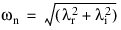
The model eigenvalues are reported to the workstation screen or in a tabular form to the tabular output (.out) file. In general, the eigenvalues are complex values, made up of real and imaginary components. The imaginary component represents the 'damped' natural frequency,  d. The damping ratio must be less than 1 in order to produce an imaginary component in the eigenvalue -- in other words, the damped natural frequency is zero whenever the damping ratio is 1 or greater.
d. The damping ratio must be less than 1 in order to produce an imaginary component in the eigenvalue -- in other words, the damped natural frequency is zero whenever the damping ratio is 1 or greater.The undamped natural frequency and damping ratio obeys following equations:

where:
■ = real part of eigenvalue.
= real part of eigenvalue. ■ = imaginary part of eigenvalues; also the damped natural frequency,
  d.
d.
= imaginary part of eigenvalues; also the damped natural frequency, d. ■ = undamped natural frequency.
= undamped natural frequency. ■ =damping ratio (
 < 1).
< 1).
=damping ratio (< 1). The relationship between the damped natural frequency,  , and undamped natural frequency,
  , is:
, is:
, and undamped natural frequency, , is: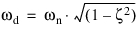
The damped natural frequency is the actual frequency at which the system is oscillating for that mode.
If you specify the COORDS, ENERGY, KINETIC, DISSIPAT, or STRAIN arguments, Adams Solver (FORTRAN) computes tabular output and writes it to the output (.out) file. For each mode in the specified range, this output could consist of up to five sections. The header section contains the mode number, undamped natural frequency, damping ratio, generalized stiffness, generalized mass and model energy for the mode. Generalized stiffness and generalized mass are in user-specified units dropping out the length dimension because the computations are done using normalized mode shapes. Hence, the generalized stiffness and the modal energy show units of User-mass/time^2.
The second section is a table of coordinates if the COORDS argument is specified. This section is not output if the COORDS argument is not specified or if the particular mode number is not within the range specified on the COORDS argument. Each part in the Adams Solver (FORTRAN) model has one row in this table. The part translational coordinates in columns labeled (x,y,z), represent the small translational displacements of the part center-of-mass (cm) marker in the global reference frame. The part rotational coordinates, in columns labeled (RX, RY, RZ), represent the small rotational displacements of the part about the global x, y and z axes, respectively. Each coordinates in this table is represented by a magnitude and a phase. The mode is normalized so that the largest component in the mode has a value of 1.0 and a phase angle of 0 degrees. Magnitude and phase of all other components in the mode are reported relative to this largest component. Phase angles are represented in the range 0 to 355 degrees. Phase angles in the range 175 to 185 degrees are reported as 180 degrees. Phase angles in the range 355 to 360 degrees as well as phase angles in the range zero to five degrees are reported as zero degrees. States of elements resulting in user supplied differential equations are also represented in the coordinate table. All components with zero magnitude are also reported as having zero phase angles.
The third section is a table of modal kinetic energy distribution if the ENERGY or KINETIC arguments are specified. This section is not present in the output for a particular mode if the mode number is not within the range of the modes specified on the ENERGY or KINETIC arguments. Each part is represented by a single row in this table. Each entry in this table represents the percentage of the total modal kinetic energy for that part in a particular direction. Translational directions in which the modal kinetic energy distribution is computed are x, y and z displacement of the part center-of-mass (cm) in the global reference frame. Rotational directions are denoted by RXX, RYY, and RZZ; these represent the small displacement rotations of the part about the global x, y and z axes, respectively. The cross rotations are represented as RXY, RYZ, and RXZ. The sum of all values in a modal energy distribution table should be 100.0. Elements resulting in user-supplied differential equations are not considered in the computation for this table.
The fourth section is a table of modal strain energy distribution if the STRAIN argument is specified. This section is not present in the output for a particular mode if the mode number is not within the range of the modes specified on the STRAIN argument. Each force element is represented by one or more rows in this table. The table below shows the contribution of various element types to this table. Computation of strain energy accounts for the direct and indirect dependence of the force on PART displacements. The indirect dependence on PART displacements may be through dependence of the force on other FORCEs, VARIABLEs, or algebraic DIFFs that may be directly or indirectly dependent on PART displacements.
Table 1. Elements Contributing to Table for Dissipative and Strain Energy Computations
Total | X | Y | Z | RX | RY | RZ | |
|---|---|---|---|---|---|---|---|
BEAM | X | X | X | X | X | X | X |
BUSHING | X | X | X | X | X | X | X |
FIELD | X | X | X | X | X | X | X |
GFORCE | X | X | X | X | X | X | X |
NFORCE for marker 1 | X | X | X | X | X | X | X |
... | X | X | X | X | X | X | X |
for marker n | X | X | X | X | X | X | X |
SFORCE (translational) | X | X | X | X | |||
SFORCE (rotational) | X | ||||||
SPRINGDAMPER (translational) | X | X | X | X | |||
SPRINGDAMPER (rotational) | X | ||||||
VFORCE | X | X | X | X | |||
VTORQUE | X | X | X | X |
In the table, X, Y, and Z refer to translation components along the global x, y and z directions and RX, RY, and RZ refer to rotational components about the global x, y and z directions. x indicates locations for contributions for individual elements. The column labeled Total contains a summation of the strain/dissipative energy contribution due to the element in various directions.
The fifth section is a table of modal dissipative energy distribution if the DISSIPAT argument is specified. This section is not present in the output for a particular mode if the mode number is not within the range of the modes specified on the DISSIPAT argument. Each force element is represented by one or more rows in this table. The table shows the contribution of elements to this table. Computation of dissipative energy accounts for the direct and indirect dependence of the force on PART velocities. The indirect dependence on PART velocities may be through dependence of the force on other FORCEs, VARIABLEs, or algebraic DIFFs that may be directly or indirectly dependent on PART velocities.
If you specify the STATEMAT argument, Adams Solver (FORTRAN) computes the state matrices representation for an Adams model. The linearized Adams model is represented as:
 =A x + B u
y = C x + D u
where:
■ represents the state variables of the plant model.
represents the state variables of the plant model.■u represents the inputs of the plant model.
■y represents the outputs from the plant model.
■A, B, C, and D are state matrices representing the plant.
You can specify the definition of plant inputs with the PINPUT argument value. Similarly, plant outputs are specified by the POUTPUT argument. Plant states are automatically determined by Adams Solver (FORTRAN) and result in the best numerical conditioning of the state matrices. While several PINPUT statements and POUTPUT statements may be present in an Adams model, you can specify only one of each on the LINEAR command.
Corresponding to each VARIABLE id specified on the PINPUT statement, a column exists in the B and D matrices. Similarly, for each VARIABLE id specified on the POUTPUT statement, a row exists in the C and D matrices. In effect, each VARIABLE id specified on the PINPUT or POUTPUT statement specifies an input or output channel, respectively.
Open-loop/closed-loop input channels are important in the computation of state matrices. If a VARIABLE statement whose id is specified on a PINPUT statement is defined as:
VARIABLE/id, FUNCTION = constant
or
VARIABLE/id, FUNCTION = function_of_time
then it is designated as an open-loop input channel. However, if the VARIABLE is of the form:
VARIABLE/id, FUNCTION=function_of_ADAMS-model-states
it is designated as a closed-loop input channel with feedback. This distinction is reflected in the A, B, and D matrices. Columns in the B and D matrices corresponding to a closed-loop input channel will have all zero values. Effects of the feedback loop due to these inputs is reflected in the A matrix. This implies that external inputs on these channels are not permitted.
Consider a system of the following form:
 =A x + B u
y = C x
Partitioning the plant input into two groups called u1 and u2, the plant model becomes:
 =A x + B1u1 + B2u2
y = C x
where B1 and B2 are sub-matrices of B, corresponding to u1 and u2, respectively; and u1 and u2 are the closed-loop and open-loop input channels, respectively.
If the input u1 represents the closed-loop input channels defined by the feedback loop:
u1 = -G y
where G is the feedback gain matrix, the plant model can then be represented as:
 = [ A - B1 G C ] x + [0] u1 + B2 u2
y = C x
Adams Solver (FORTRAN) computes the state matrices for a model with this combination of inputs and outputs as:
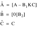
The effects of the closed-loop channels are reflected in the  matrix. Columns of the
  matrix corresponding to the closed-loop channel are zero. In other words, the PINPUT or POUTPUT id specification that you choose on the LINEAR command affects the structure of the A, B, C, and D matrices.
matrix. Columns of the matrix corresponding to the closed-loop channel are zero. In other words, the PINPUT or POUTPUT id specification that you choose on the LINEAR command affects the structure of the A, B, C, and D matrices.Tip: | ■To reduce computing time, specify the NOVECTOR argument with the EIGENSOL argument if mode shapes are not desired. ■Specify the LINEAR command to assess stability of Adams models by computing its eigenvalues. Eigenvalues with positive real parts correspond to unstable modes of the system. ■If you specify the PINPUT and the POUTPUT arguments for state matrices output, Adams Solver (FORTRAN) produces all four matrices (A, B, C, and D). If you do not specify the PINPUT argument, Adams Solver (FORTRAN) does not produce the B or D matrices. Similarly, if you do not specify the POUTPUT argument, Adams Solver (FORTRAN) will not produce the C or D matrices. If you do not specify either the PINPUT or POUTPUT arguments, Adams Solver (FORTRAN) produces only the A matrix. ■You may define several PINPUT and POUTPUT statements in an Adams Solver (FORTRAN) dataset, however, a LINEAR command allows only one PINPUT and one POUTPUT statement to be specified at a time. If you issue a series of LINEAR commands, Adams Solver (FORTRAN) computes alternate state matrix descriptions at the same operating point with different combinations of PINPUT and POUTPUT identifiers. Changes in the PINPUT and POUTPUT descriptions are reflected in the A, B, C, and D matrices. |
Caution: | ■The LINEAR command may only be issued following a STATIC, DYNAMIC, or TRANSIENT analysis. ■Dependence of function expressions on joint reaction forces is ignored for linearization. ■Adams models containing nonholonomic UCONs cannot be linearized. ■Since the eigensolution and state matrices characterize behavior of the nonlinear Adams model in a neighborhood of the operating point, you should assess if an operating point is at a suitable point about which to linearize the system equations. A model can always be linearized about its static position. Decide whether or not to linearize models undergoing motion. Three situations to consider are listed below. ■All or some parts in the Adams model have translational but no angular velocities. It is acceptable to linearize models at such operating points. ■In addition to translation velocities, all or some parts in the Adams model have angular velocities. If the angular velocity vector passes through the center of mass of the respective parts, it is acceptable to linearize such models. An example of such a system would be a vehicle moving in a straight line with its wheels rotating about their axes. ■If, however, the angular velocity vector does not pass through the center of mass of the respective part, the system should not be linearized. This is especially true if the angular velocity magnitudes are large. An example of this would be a spinning, articulated structure containing a center hub with articulated outboard parts. The spin axes of the outboard parts do not pass through the center of mass of the parts. Linearization of such models may produce spurious results. ■Applying MOTION to a JOINT restricts the respective degree-of-freedom. As a result, during state matrices output, any PINPUT applied to a part constrained by such a MOTION results in a zero column for the B matrix. |
Advanced eigensolution issues
In case you need to compare the computed eigensolution with results from another software package, you may export the linearization matrices using the LINEAR/STATEMAT option. The exported [A] matrix is the one we send to the eigensolver.
In general, the issues affecting the quality of the eigensolution are the following:
a. Models in singular configurations. Models in singular configuration may report spurious modes and frequencies or they may report different values (with a sign reverse) under small perturbations.
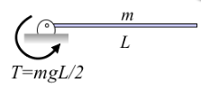
For instance, the beam shown in the figure above is at an unstable equilibrium position. A small perturbation moving the tip downward will cause the torque to restore the previous equilibrium position (complex eigenvalue). However, a small perturbation moving the tip upward will case the system to move away from the horizontal position (real eigenvalue). At exactly the horizontal position the eigenvalues are zero. Solving a complex system with the same overall topology may results in spurious eigenvalues.
b. Accelerating models. Accelerating or rotating components usually involve mode shapes involving velocity states and may show strange mode shapes.
c. Multiple rigid body modes. If the model has the potential to experiment rigid body motion, the eigensolver may show up with noisy frequencies instead of a zero value. This depends on the size of the model. Moreover, if the model has DIFFs or LSEs or GSEs or TFSISOs objects, then some modes will be related to the differential states with almost no coupling with overall motion of the system. Those modes will show no animation.
d. Overdamped models. Damping may create spurious modes that create clutter and make difficult to find the modes of interest. Since the damping is hard to estimate, we recommend also running the eigensolution with the NODAMP option to gain perspective on the interesting modes. Damping can be added afterward to estimate its influence in the solution.
e. Friction in stiction regime. If the model has FRICTION objects running in the stiction mode, you may get spurious frequencies and mode shapes due to the stiffness of the force element added to model the stiction.
f. Numerical limitations. In general, the linearization matrix [A] is non-symmetric, ill-conditioned and sparse. In addition, there is a natural limitation in the precision of the arithmetic operations of the computer. The end results may be that frequencies and mode shapes may include noisy results especially in both the lower end of the real eigenvalues (real-only eigenvalues with small values) and in the lower imaginary spectrum (complex eigenvalues with small imaginary part). Higher real-only eigenvalues and higher imaginary eigenvalues are usually better extracted.
6. Examples
LINEAR/EIGENSOL
This command computes an eigenanalysis for the Adams model. Adams Solver (FORTRAN) writes the eigenvalues and mode shapes to the Results file where they can be read and displayed by a postprocessor such as Adams View.
LINEAR/STATEMAT, PINPUT=10, POUTPUT=20
, FORMAT=MATRIXX FILE=STATES.MAT
, FORMAT=MATRIXX FILE=STATES.MAT
This command computes state matrices for the Adams model, using PINPUT/10 as inputs and POUTPUT/20 as outputs. The state matrices are written to file STATES.MAT in MATRIXX format.
7. Applications
Eigensolutions provide you with information that may be used in assessing stability of the Adams model. If you import control systems descriptions or distributed elasticity data from external sources, you can verify the stability of their Adams models.
1. Eigendata computed by Adams Solver (FORTRAN) can be used to validate Adams models against eigendata from external sources.
2. State matrices descriptions can be used in designing control systems for Adams models. This description is suitable for computing frequency response data in matrix manipulation software packages (see the PINPUT, POUTPUT, and VARIABLE statements).
3. State matrices output by Adams Solver (FORTRAN) in the MATRIXX format are suitable for being read into a second Adams model with a MATRIX statement. These matrices can form the definition of a dynamical system defined by an LSE statement in the second Adams model.
7.1 Eigenanalysis Application
Consider a model of an inverted pendulum on a sliding cart as shown in Figure 6 below. The listing of the Adams Solver (FORTRAN) dataset for this model is shown in Listing 1.
Figure 6 Inverted Pendulum on Sliding Cart Model
The sliding cart in this model is represented by PART/1 and the inverted pendulum is represented by PART/2. PART/1 slides along the global x axis in translational joint, JOINT/1, while PART/2 can rotate about the axis of revolute joint, JOINT/2. PART/1 is connected to ground by a SPRINGDAMPER/1. TFSISO/1 represents an actuator connected between PART/1 and PART/2. Force generated by this actuator is applied on the two parts by SFORCE/1. No input is applied to the actuator for the present. To assess stability of this model, execution of Adams Solver (FORTRAN) is initiated. Once Adams Solver (FORTRAN) verifies that the model data is syntactically correct, issue the SIMULATE/STATIC command. On achieving static equilibrium, issue the LINEAR/EIGEN command. Eigenvalues reported by Adams Solver (FORTRAN) are shown in Table 2 below.
Table 2. Model Eigenvalues
EIGENVALUES | ||
Number | Real (cycles/unit time) | Imag. (cycles/unit time) |
1 | 5.00909210E-02 | 0.00000000E+00 |
2 | -5.00924580E-02 | 0.00000000E+00 |
3 | -3.18309800E+01 | 0.00000000E+00 |
4 | -3.17994185E-01 | +/- 6.36188992E-01 |
The table shows that the system has three stable and one unstable mode. To determine the cause of this instability, use the data produced by Adams Solver (FORTRAN) (.res, .adm, and so on) in Adams to display the deformed mode shapes of the model.
Figure 7 (a) and (b) show mode shapes for mode 1, which is unstable, and mode 4, which is stable.
Figure 7 Deformed Mode Shape 1(a) and Deformed Mode Shape 4 (b)
Figure 7 (a) shows that PART/1 is essentially stationary while PART/2 is moving. You can conclude that PART/2 is the cause of the instability in this model. This is an expected result for this model, since the inverted pendulum is at an unstable operating point. It is obvious that disturbing the pendulum will cause it to swing about the revolute joint axis.
As illustrated by this example, viewing mode shapes in a graphical display can provide very significant insight into the dynamic behavior of the model. In complicated Adams models, this insight is vital in understanding the model dynamics. In Example 2: State Matrices Output below, based on the state matrices computed for this model, a feedback control law will be designed to stabilize this model.
7.2 State Matrices Output
Design and implementation of a control system for an Adams model is described in this example. The plant model used in this example is identical to the Adams model described in Example 1. The purpose of the control design exercise is to design a feedback controller to attempt to stabilize the inverted pendulum Adams model described in Example 1. For control design purposes, the state matrix representation of the Adams model is required and is generated by the LINEAR/STATEMAT command.
Stabilization of this model requires that PART/2 maintain its inverted vertical position despite external disturbances applied on it. External disturbances considered here are gravity acting vertically downwards and an external force applied to the pendulum in the x-direction. On sensing a deviation of the pendulum from the desired position, the control law determines an appropriate signal to apply to actuator TFSISO/1 to restore PART/2 to its desired position. The control law operates on the basis of measuring output signals from the plant and then computes a signal to apply to the actuator.
As shown in Figure 8 for the present model, 3 signals are output by the plant. VARIABLE/10 is a measurement of the relative x displacement between PART/1 and PART/2. VARIABLE/20 is a measurement of the relative x velocities between the two parts. VARIABLE/30 is the integral of the relative x displacements between the two parts. These 3 signals are designated as outputs from the plant by POUTPUT/1.
Input to the plant, that is, input signal to the actuator, is defined as VARIABLE/2. This is designated as input to the plant by PINPUT/1. Adams Solver (FORTRAN) implementation of the input/output structure and the external disturbances is shown in Listing 2: Plant Input/output Specification . This implementation, when combined with the plant model as shown in dataset 1 in FILE=c results in the open-loop model. When the open-loop model is complete, an Adams Solver (FORTRAN) execution session is initiated.
Figure 8 Open-Loop Model
The model is read into Adams Solver (FORTRAN). After Adams Solver (FORTRAN) verifies the model data syntax, issue the SIMULATE/STATIC command to determine the equilibrium position. On achieving the equilibrium position, issue the LINEAR/EIGEN, NOVECTOR command to verify the eigenvalues of the model. The next table shows the eigenvalues for the open-loop model.
Table 3. Open-Loop Eigenvalues
EIGENVALUES | ||
Number | Real (cycles/unit time) | Imag. (cycles/unit time) |
1 | -2.66440631E-17 | 0.00000000E+00 |
2 | 5.00909210E-02 | 0.00000000E+00 |
3 | -5.00924580E-02 | 0.00000000E+00 |
4 | -3.18309800E+01 | 0.00000000E+00 |
5 | -3.17994185E-01 | +/- 6.36188992E-01 |
The table shows that the open-loop model has one eigenvalue more than the model in Example 1: Eigenanalysis Application This is due to the introduction of the relative displacement integrator TFSISO/2 in the open-loop model. To linearize the model and compute the state matrices, issue the LINEAR/STATEMAT, PINPUT=1, POUTPUT=1, file=adams.mat command. Adams Solver (FORTRAN) linearizes the model and writes the state matrices in the default format to adams.mat file. Contents of the ADAMS.MAT file are in Listing 3: State Matrices (FSAVE Format) for the Open-Loop Model. The Adams Solver (FORTRAN) session then terminates. You may design a controller by reading the ADAMS.MAT file into the control design package exercising various control design methodologies. The description of the control design step is beyond the scope of the present document. A text on this subject or documentation for control design software packages should be consulted for further details.
Now that the feedback control has been designed, it needs to be implemented in Adams Solver (FORTRAN) for a closed-loop simulation. The controller designed for this example is a dynamic compensator. As shown in Figure 4 below, this is implemented in Adams Solver (FORTRAN) as LSE/1. The A, B and C matrices associated with this LSE are defined by MATRIX/100, 200, and 300, respectively. Adams Solver (FORTRAN) reads the data for these matrices from a file named incomp.dat. To connect this feedback compensator to the plant model, inputs to LSE/1, ARRAY/303 are connected to outputs from the plant model. Also, ARRAY/1, which is input to the actuator, TFSISO/1, is now defined as the output from the compensator, VARIABLE/2. This completes the closed-loop Adams model. The complete Adams Solver (FORTRAN) dataset for this model is shown in dataset 3 and dataset 4.
Figure 9 Closed-Loop Model
To verify and simulate the closed-loop model, an Adams Solver (FORTRAN) simulation is initiated. The closed-loop model is first equilibrated in its static position. The eigenvalues for this model are computed and represented in Table 4 shown next.
Table 4. Closed-Loop Eigenvalues
EIGENVALUES | ||
Number | Real (cycles/unit time) | Imag. (cycles/unit time) |
1 | -5.35233760E-01 | 0.00000000E+00 |
2 | -3.18270747E+01 | 0.00000000E+00 |
3 | -2.37397000E-01 | +/- 7.54488218E-02 |
4 | -7.37798519E-03 | +/- 1.51611302E-01 |
5 | -5.47796070E-01 | +/- 5.12745191E-01 |
6 | -2.43466412E-01 | +/- 5.71313964E-01 |
7 | -2.46528313E+01 | +/- 1.00614794E+01 |
Table 4 above shows that the closed-loop model is stable. The closed-loop model has more eigenvalues than the open-loop model. This is due to the dynamical state variables introduced by LSE/1. Eigenvalues for the closed-loop Adams model can be compared with the closed-loop eigenvalues computed in the control design package. Now that the stability properties of the closed-loop Adams model have been verified, it can be simulated to obtain its dynamic response. The time profile of the external disturbance is as shown in Figure 10. The closed-loop model response to external disturbance is as shown in Figure 11. As illustrated in this figure, the closed-loop model provides complete disturbance rejection for displacement of PART/2.
Figure 10 Time Profile of External Disturbance
Figure 11 Closed-Loop System Response
The input signal applied to the actuator and the force generated by the actuator are shown in Figure 12 and Figure 13, respectively.
Figure 12 Input Signal to Actuator
Figure 13 Force Generated by Actuator
The process of control design and simulation is an iterative one. If the closed-loop system does not perform as expected, the control design specifications may have to be changed and a new controller designed to achieve better performance.
7.2.1 State Matrices Output Format
MATRIXX Format
State matrices output by Adams Solver (FORTRAN) in the MATRIXX format conforms to the MATRIXx FSAVE ASCII file specification. These specifications are given in the Xmath Basics Guide, 1996, Integrated Systems Inc., Santa Clara, CA.
More than one matrix may be present in a single file. The Adams Solver (FORTRAN) state matrices file can have up to seven matrices. The first four matrices are the A, B, C, and D state matrices. The next three matrices are STATES, PINPUT, and POUTPUT. The contents and format of these matrices are explained in Contents of the STATES, PINPUT, and POUTPUT Matrices.
MATLAB Format
State matrices output by Adams Solver (FORTRAN) in the MATLAB format conform to the ASCII flat file format. This format requires that all entries in a row of the matrix be written in a single record. Successive values in a row are separated by a single space. A file is allowed to contain only one matrix. Therefore, Adams Solver (FORTRAN) may create up to seven output files, one each for the A, B, C, and D matrices, one for STATES, one for PINPUT, and one for POUTPUT. The contents and format of the last three matrices are as shown in Contents of the STATES, PINPUT, and POUTPUT Matrices. The file name you specify is used as a base name and is appended with the matrix name to write the matrix of the appropriate type. The file names used for the seven matrices are as given in Table 5 below.
Table 5. File Names Used for MATLAB State Matrices Output
Matrix name | File Name |
|---|---|
A | "base_name" "a" |
B | "base_name" "b" |
C | "base_name" "c" |
D | "base_name" "d" |
STATES | "base_name" "st" |
PINPUT | "base_name" "pi" |
POUTPUT | "base_name" "po" |
7.2.2 Contents of the STATES, PINPUT, and POUTPUT Matrices
STATES Matrix
The STATES matrix contains information regarding states that Adams Solver (FORTRAN) has chosen for the state matrices representation. For each state, one record exists in this matrix. The following information is contained in each record:
Type_of_element | Element_identifier | Element_coordinate |
Type_of_element
Type_of_element can take on the following values:
1. Part coordinates
2. States in a LSE element
3. States in a TFSISO element
4. States in a GSE element
5. Diff variable
6. Coordinate for a PTCV element
7. Coordinates for a CVCV element
8. FLEX_BODY element
9. POINT_MASS element
Element_identifier
Element_identifier is the eight-digit Adams Solver (FORTRAN) identifier of the element.
Element_coordinate
If Type_of_element=1, the Element_coordinate can take on the values:
1. x-displacement
2. y-displacement
3. z-displacement
4.  angle of part principal axis
angle of part principal axis 5.  angle of part principal axis
angle of part principal axis 6.  angle of angle of part principal axis
angle of angle of part principal axis 7. 
8. 
9. 
10. 
11. 
12. 
For Type_of_element=2 to 5, Element_coordinate is the sequence number in the set of states defining that element.
For Type_of_element=6, the only permissible value for Element_coordinate is 1, that is, the alpha parameter value that defines the contact point on the curve.
For Type_of_element=7, Element_coordinate may take on the value of 1 or 2, representing the parameter values for the first (I) or second (J) curve in a CVCV statement that defines the contact point on the curve.
For Type_of_Element=8, the Element_coordinate can take on the values:
1 - 12 same as for Type_of_Element=1
1 E6 + n nth modal generalized coordinate
2 E6 + n first time derivative of the nth modal generalized coordinate
1 E6 + n nth modal generalized coordinate
2 E6 + n first time derivative of the nth modal generalized coordinate
For Type_of_Element=9, the Element_coordinate can take on the following values:
1 - 3 same as for Type_of_Element=1
4
5
6
4
5
6
In the MATRIXX format, this data is organized in column order form so that the STATES matrix contains three rows and number of columns is equal to the number of states in the model. In the MATLAB format, this data is organized in the row order form. Therefore, the STATES file contains data organized in the three columns and the number of rows is equal to the number of states in the model.
7.2.3 PINPUT and POUTPUT Matrices
The first record in the PINPUT/POUTPUT data contains the Adams Solver (FORTRAN) identifier of the PINPUT/POUTPUT statement, respectively, that was used on the LINEAR command to generate these state matrices. Subsequent records contain the Adams Solver (FORTRAN) identifiers of the VARIABLE statement identifiers used on these statements. In the MATRIXX as well as the MATLAB format, this data is organized as a matrix with 1 column and number of rows equal to one plus the number of variables on the PINPUT or POUTPUT statement.
All data for the STATES, PINPUT, and POUTPUT matrices is written as floating point data.
8. Appendix
Listing 1: Inverted Pendulum Model
ADAMS Inverted pendulum model.
!
pa/99, ground
ma/99,qp=0,0,0, zp =1,0,0
!
! ===> Sliding cart <===
pa/1,ma=10,ip=10,10,10,cm=10
ma/10,qp=5,0,0 ! CM marker.
ma/11,qp=5,0,2, zp=5,1,2 ! revolute joint marker.
ma/12,qp=3,-2,-2 ! graphics marker.
ma/13,qp=5,0,0, zp=6,0,0 ! translational joint marker.
ma/14,qp=5,0,12
ma/15,qp=12,0,2 ! actutator attachment point
!
! ===> Inverted pendulum <===
pa/2,ma=1,cm=20, ip=1,1,1
ma/20,qp=5,0,12 ! CM marker.
ma/21,qp=5,0,2, zp=5,1,2 ! revolute joint marker.
ma/22,qp=5,0,12, zp=5,1,12 ! graphics marker.
ma/23,qp=5,0,7 ! actutator attachment point
ma/24,qp=5,0,2, zp=5,0,3 ! graphics marker.
!
joint/1,tran,i=13,j=99
joint/2,rev,i=11,j=21
!
! ===> Spring damper between cart and ground <===
springdamper/1,tran,i=99,j=13,k=200,c=40,l=5
!
gra/2, circle,cm=20, r=1.5,seg=20
gra/3, circle,cm=22, r=1.5,seg=20
gra/4, cylind,cm=24, l=8.5, r=0.25,seg=10,side=10
gra/5, box, corn=12, x=9, y=4, z=4
!
! ===> External disturbance <===
sforce/1001, i=20, j=99, action, tran,
,fun=step(time,0,0,.5,10)-step(time,1,0,1.5,10)
!
! ===>Actuator Dynamics<===
tfsiso/1,num=10, den=1,0.005
,u=1,x=2,y=3
array/1,u,var=2 ! input signal to actuator
array/2,x ! actuator state
array/3,y ! force generated by actuator.
!
! ===>Actuator force<===
sforce/1,i=15,j=23, trans,
,function=aryval(3,1)
!
! ===>Input to Actuator<===
vari/2,fun=0
!
accgrav/kg=-1
result/format
!
end
Listing 2: Plant Input/output Specification
! ===> PLANT INPUT/OUTPUT definition <===
! -------------------
!
var/1,fun=dx(20,14)
Displacement integrator
tfsiso/2, num=1, den=0,1
,u=20,x=21,y=22
array/20, U, VAR=1
array/21, X
array/22, Y
!
! ===> Outputs <===
vari/10, function= varval(1) ! displacement
vari/20, function= vx(20,14) ! velocity
vari/30, function= aryval(22,1) ! displ. integrated
!
!
! ===> Plant input designation <===
pinput/1,var=2
!
! ===> Plant output designation <===
poutput/1,var=10,20,30
!
Listing 3:State Matrices (FSAVE Format) for the Open-Loop Model
FSAVE
A 6 6B 6 1C 3 6D 3 1
STATES 3 6PINPUT 2 1POUTPUT 4 1
A 6 6 0(3(1PE25.17))
-3.99604352126607320E+00 1.00000000000000000E+00 -3.95647873392680550E-02
0.00000000000000000E+00 0.00000000000000000E+00 0.00000000000000000E+00
-1.99703264094955490E+01 0.00000000000000000E+00 -2.96735905044510420E-01
0.00000000000000000E+00 0.00000000000000000E+00 -9.99999999962142390E-01
0.00000000000000000E+00 0.00000000000000000E+00 0.00000000000000000E+00
1.00000000000000000E+00 0.00000000000000000E+00 0.00000000000000000E+00
-9.89119683481701380E-03 0.00000000000000000E+00 9.89119683481701210E-02
0.00000000000000000E+00 0.00000000000000000E+00 9.99999999962142390E-01
4.02439896739235910E-02 0.00000000000000000E+00 -4.02439896739235860E-01
0.00000000000000000E+00 -2.00000000000000000E+02 0.00000000000000000E+00
0.00000000000000000E+00 0.00000000000000000E+00 0.00000000000000000E+00
0.00000000000000000E+00 0.00000000000000000E+00 0.00000000000000000E+00
B 6 1 0(3(1PE25.17)
0.00000000000000000E+00 0.00000000000000000E+00 0.00000000000000000E+00
0.00000000000000000E+00 2.00000000000000000E+03 0.00000000000000000E+00
C 3 6 0(3(1PE25.17))
0.00000000000000000E+00 -1.00000000000000000E+00 0.00000000000000000E+00
-9.99999999962142390E-01 0.00000000000000000E+00 0.00000000000000000E+00
0.00000000000000000E+00 1.00000000000000000E+00 0.00000000000000000E+00
9.99999999962142390E-01 0.00000000000000000E+00 0.00000000000000000E+00
0.00000000000000000E+00 0.00000000000000000E+00 0.00000000000000000E+00
0.00000000000000000E+00 0.00000000000000000E+00 1.00000000000000000E+00
D 3 1 0(3(1PE25.17))
0.00000000000000000E+00 0.00000000000000000E+00 0.00000000000000000E+00
STATES 3 6 0(3(1PE25.17))
1.00000000000000000E+00 1.00000000000000000E+00 7.00000000000000000E+00
1.00000000000000000E+00 1.00000000000000000E+00 1.00000000000000000E+00
1.00000000000000000E+00 2.00000000000000000E+00 7.00000000000000000E+00
1.00000000000000000E+00 2.00000000000000000E+00 1.00000000000000000E+00
3.00000000000000000E+00 1.00000000000000000E+00 1.00000000000000000E+00
3.00000000000000000E+00 2.00000000000000000E+00 1.00000000000000000E+00
PINPUT 2 1 0(3(1PE25.17))
1.00000000000000000E+00 2.00000000000000000E+00
POUTPUT 4 1 0(3(1PE25.17))
1.00000000000000000E+00 1.00000000000000000E+01 2.00000000000000000E+01
3.00000000000000000E+01
Listing 4: Closed-Loop Model
ADAMS Inverted pendulum closed-loop model.
!
pa/99, ground
ma/99,qp=0,0,0, zp =1,0,0
!
! ===> Sliding cart <===
pa/1,ma=10,ip=10,10,10,cm=10
ma/10,qp=5,0,0 ! CM marker.
ma/11,qp=5,0,2, zp=5,1,2 ! revolute joint marker.
ma/12,qp=3,-2,-2 ! graphics marker.
ma/13,qp=5,0,0, zp=6,0,0 ! translational joint marker.
ma/14,qp=5,0,12
ma/15,qp=12,0,2 ! actutator attachment point
!
! ===> Inverted pendulum <===
pa/2,ma=1,cm=20, ip=1,1,1
ma/20,qp=5,0,12 ! CM marker.
ma/21,qp=5,0,2, zp=5,1,2 ! revolute joint marker.
ma/22,qp=5,0,12, zp=5,1,12 ! graphics marker.
ma/23,qp=5,0,7 ! actutator attachment point
ma/24,qp=5,0,2, zp=5,0,3 ! graphics marker.
!
joint/1,tran,i=13,j=99
joint/2,rev,i=11,j=21
!
! ===> Spring damper between cart and ground <===
springdamper/1,tran,i=99,j=13,k=200,c=40,l=5
!
gra/2, circle,cm=20, r=2,seg=10
gra/3, circle,cm=22, r=2,seg=10
gra/4, cylind,cm=24, l=8, r=0.5,seg=10,side=10
gra/5, box, corn=12, x=9, y=4, z=4
!
! ===> External disturbance <===
sforce/1001, i=20, j=99, action, tran,
,fun=step(time,0,0,.5,10)-step(time,1,0,1.5,10)
!
! ===>Actuator Dynamics<===
tfsiso/1,num=10, den=1,0.005
,u=1,x=2,y=3
array/1,u,var=2 ! input signal to actuator
array/2,x ! actuator state
array/3,y ! force generated by actuator.
!
! ===>Actuator force<===
sforce/1,i=15,j=23, trans,
,function=aryval(3,1)
!
!
! ===> PLANT INPUT/OUTPUT definition <===
! -------------------
!
var/1,fun=dx(20,14)
Displacement integrator
tfsiso/2, num=1, den=0,1
,u=20,x=21,y=22
array/20, u, var=1
array/21, x
array/22, y
!
! ===> Outputs <===
vari/10, function= varval(1) ! displacement
vari/20, function= vx(20,14) ! velocity
vari/30, function= aryval(22,1) ! displ. integrated
!
!
! ===> Plant input designation <===
pinput/1,var=2
!
! ===> Plant output designation <===
poutput/1,var=10,20,30
!
! ===>Feedback compensator<===
! --------------------
!
lse/1,a=100, b=200, c=300,
,x=101,y=202,u=303,ic=404
!
array/101, x ! compensator state
array/202, y ! compensator output
array/303, u, var= 10, 20, 30 ! compensator input
array/404, ic, num=0,0,0,0,0,0
!
matrix/100,
,file=incomp.mat, name=ac
matrix/200,
,file=incomp.mat, name=bc
matrix/300,
,file=incomp.mat, name=cc1
!
! ===> Feedback signal from compensator to actuator <===
variable/2, fun=-aryval(202,1)
!
accgrav/kg=-1
result/format
!
end
Listing 5: "incomp.mat" Input Data file
MATRIXx VERSION 700 3 04-OCT-91 15:27
AC 6 6BC 6 3CC1 1 6
AC 6 6 0(1P3E25.17)
-1.00799962154710574E+01 9.75162440467575053E-01 9.98460749273361898E+01
9.61406957584617916E-01 3.11437948419828955E-03 -1.78574044858736743E+04
-8.50683303123077716E-01 -4.98921809045884790E-01 1.01587769607181722E+00
1.14325442554075640E+00 -4.49484043101296749E-01 -1.69576019090885748E+04
9.98009512743940519E+00 2.48375595324249708E-02 -9.98470640470196713E+01
3.85930424153820839E-02 -3.11437948419828955E-03 1.79036593612407414E+04
-1.48327577193440696E-01 4.98921809045884790E-01 -1.02576889290663420E+00
-1.14325442554075640E+00 4.49484043101296749E-01 1.74318979368853470E+04
-1.20450308829068348E-01 7.73595535159733033E-02 -1.23564688768258060E-01
-4.73156382486152438E-01 -1.34087821455120393E+00 2.82840625758381648E+04
4.02439896739235914E-02 0.00000000000000000E+00 -4.02439896739235858E-01
0.00000000000000000E+00 0.00000000000000000E+00 -2.09248210623341492E+02
BC 6 3 0(1P3E25.17)
1.38436380363864547E-01 -4.98921809064772792E-01 1.12468086129738198E+00
1.14325442558403734E+00 5.50515956881686863E-01 -9.30005800767228163E-01
-9.98009512743940519E+00 -2.48375595324249708E-02 9.98470640470196713E+01
9.61406957584617916E-01 3.11437948419828955E-03 -1.36246052474731605E+04
1.20450308829068348E-01 -7.73595535159733033E-02 1.23564688768258060E-01
4.73156382486152438E-01 1.34087821455120393E+00 2.08671855656208993E-01
CC1 1 6 0(1P3E25.17)
2.11639961920025588E+00 8.47833595164392051E+00 -2.13952705688378986E+00
-8.71548396554230820E+00 -1.41421356238469098E+01 4.62410531167074812E-03
See other Simulation available.