FE_PART
The FE_PART statement defines a set of finite elements with distributed mass. The finite elements are fully embedded in the solution process, in other words, Adams Solver assembles the governing equations and solves the corresponding governing finite elements equations that are coupled to the standard multibody dynamic equations.
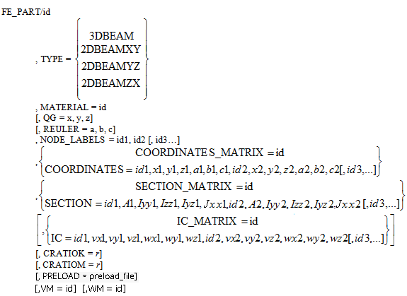
The TYPE of FE_PART specifies whether this set of elements is use to model 3D beam and 2D beam and so on.
Format
Arguments
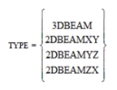 | Specifies the type of finite element. A 3DBEAM is finite element beam modeled using the Absolute Nodal Coordinate Formulation (ANCF). It has advantages versus standard finite elements found in Nastran, namely it is suited to fit multibody dynamics codes like Adams providing full geometrically nonlinear behavior. See references for selected papers. The 2DBEAMXY, 2DBEAMYZ and 2DBEAMZX are special cases of 3DBEAM when the beam has a planar behavior. Like 2D PARTS, they may have an offset and they assemble a reduced set of equations of motion. |
QG=x, y, z | Defines the Cartesian initial coordinates of the origin of the body coordinate system (BCS) with respect to the global coordinate system (GCS). |
REULER=a, b, c | Defines the 3-1-3 Euler angles that Adams Solver (C++) uses to establish the initial orientation of the BCS with respect to the coordinate system. The a, b, and c rotations are in radians and are, respectively, about the z-axis of ground, the new x-axis, and the new z-axis of the BCS. To input Euler angles in degrees, add a D after each value. |
MATERIAL = id | Specifies the identifier of the MATERIAL statement used by this element. |
NODE_LABELS=id1, id2 [, id3…] | Specifies the list of nodes used by this element to define its geometry. Straight beams may only require two nodes to completely define the element. However, if cross sectional properties change along the axis of the beam, or if the beam is curved, users may want to use more than two nodes to define the beam. Adding more nodes adds more equations of motion but provides better modeling of the real system. The list of nodes provides the sequence in which the nodes are connected forming the beam. Each node defines a coordinate system. Each pair of nodes defines a beam like finite element using the ANCF (Absolute Nodal Coordinate Framework) element. The elements are curved following a polynomial interpolation. |
COORDINATES_MATRIX=id | Specifies the identifier of the MATRIX statement holding the nodal information for this element. The MATRIX must have 7 columns. Each row must include an integer defining a node (that is, node ID) and 6 coordinates specifying the location and orientation of the node with respect to the BCS of the element. The node IDs defined in this statement are the nodes used in the NODES option. |
COORDINATES=id1, x1,… | Specifies a list of values. The values are arranged in sets of 7 values each. The first in the set is an integers (defining a node ID) followed by 6 coordinates specifying the location and orientation of the node with respect to the BCS of the element. The node IDs defined in this statement are the nodes used in the NODES option. |
SECTION_MATRIX=id | Specifies the identifier of the MATRIX statement holding the cross section property values for each node. The MATRIX must have 6 columns. Each row must include an integer corresponding to a node ID and 5 values defining the Area, Iyy, Izz, Iyz and Jxx of the beam at the set node. See Note 1 below. |
SECTION = id1, A1,… | Specifies a list of values. The values are arranged in sets of 6 values each. The first in the set is an integer specifying a node ID. The next 5 values are the Area, Iyy, Izz, Iyz and Jxx of the beam at the specified node. See Note 1 below. |
IC_MATRIX=id | Specifies the identifier of the MATRIX statement holding the velocity initial conditions at each node. The MATRIX must have 7 columns. Each row starts with an integer corresponding to a node ID and 6 values defining the initial velocities(vx,vy,vz,wx,wy,wz) of the set node with respect to the BCS or if specified, VM and/or WM. All six values for all nodes of the FE Part must be specified. |
IC=id1, vx1,… | Specifies a list of values. The values are arranged in sets of 7 values each. The first in the set is an integer (a node ID) followed by 6 coordinates (vx,vy,vz,wx,wy,wz) specifying the initial velocities of the set node with respect to the BCS or if specified, VM and/or WM. All six values for all nodes of the FE Part must be specified. Initial rotational velocities (wx,wy,wz) are specified in radians per second. |
CRATIOK=r | Specifies the fraction of the stiffness matrix that contributes to the damping matrix for this element. Note: The CRATIOK and CRATIOM used in the FE part damping are same as those in the Rayleigh damping; however, it should be noted that since the FE part formulation includes geometrical nonlinearity, the stiffness matrix and mass matrix are not constant (except for the 2D FE part). So, the CRATIOM and CRATIOK is multiplied to the instantaneous mass matrix and the instantaneous stiffness matrix (that is, tangent stiffness matrix) respectively. |
CRATIOM=r | Specifies the fraction of the mass matrix that contributes to the damping matrix for this element. Note: The CRATIOK and CRATIOM used in the FE part damping are same as those in the Rayleigh damping; however, it should be noted that since the FE part formulation includes geometrical nonlinearity, the stiffness matrix and mass matrix are not constant (except for the 2D FE part). So, the CRATIOM and CRATIOK is multiplied to the instantaneous mass matrix and the instantaneous stiffness matrix (that is, tangent stiffness matrix) respectively. |
PRELOAD = preload_file | Specifies the name of a file containing preloaded conditions information for this fe_part. |
VM = id | Specifies the identifier of the marker that specifies the direction of the translational components of initial velocity defined in the IC or IC_MATRIX. VM defaults to the FE Part BCS. |
WM=id | Specifies the identifier of the marker that specifies the axes about which angular velocity initial condition (wx,wy,wz) are defined. WM defaults to the BCS location (QG) and orientation (REULER). The origin of the WM marker lies on the axis of rotation. This is useful for rotating systems. |
Notes: | 1. Iyy, Izz and Iyz are the area moments of the cross section around the nodal Y and Z axes defined by the node information. Iyz is the product of inertia. Jxx is the torsional constant which is used to assemble the torsional equation of motion. The warping deformation is not considered here. 2. The number of nodes used, n, determines the number of degrees of freedom (DOF) of the FE Part as such: DOF for 3DBeam : = 3*((4*number_of_nodes)-1), DOF of 2DBeams : = 4*(number_of_nodes) |
Extended definition for beams
The nodes define the neutral axis of the beam. The neutral axis passes through the origin of each node. All nodes must be oriented such that the positive x-axis is tangent to the neutral axis of the beam (centroid).
For simple uniform beam, two nodes are usually enough to model it. However, if the cross section properties change along the axis, or if the beam is curved, users need to use more nodes. If the user decides to use more nodes, then additional degrees of freedom are assigned to the element making it more accurate in modeling the real system. If more than two nodes are used, the beam in fact becomes a set of finite elements.
One limitation of FE Part beams is that the shear center is assumed coincident with the neutral axis.
Each node defines a nodal coordinate system. This coordinate system has three purposes: the origin defines the location of the neutral axis of the beam, that is, the location of the center of mass of the cross section. Second, the x-axis defines normal to the cross section. Third, the other axes are used to define the cross sectional properties and the rendering of graphics representing the cross section geometry.
See section FAQ for more information.
References
1. Gerstmayr, J. and Shaban, A. "Analysis of higher and lower elements for the Absolute Nodal Coordinate Formulation". Proceedings of IDETC/CIE 2005.
2. Simo, J. and Vu-Quoc, L. "A Geometrically-exact rod model incorporating shear and torsion-warping deformation", J. Solids Structures Vol 27, No3, pp 371-393, 1991.
3. Berzeri, M. and Shabana, A. "Development of simple model for the elastic forces in the absolute nodal co-ordinate formulation". Journal of Sound and Vibration (2000) 235(4), 539-565.
1. Example
A distributed-mass beam is shown in Figure 12 below. For this case, just two nodes are enough to model the beam.
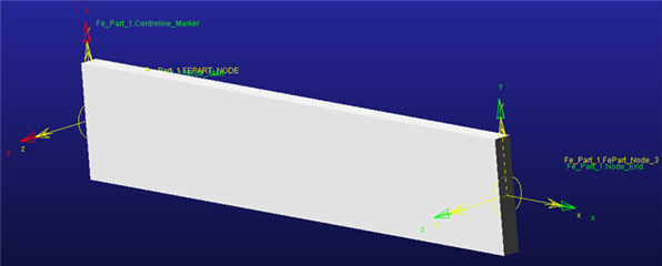
Figure 12 A simple beam
FE_PART/1
, TYPE = 3DBEAM
, QG = 130, 50, 0
, NODE_LABELS = 7, 77
, COORDINATES=
, 7, 0, 0, 0, 0, 0, 0
, 77, 6.5, 0, 0, 0, 0, 0
, SECTION=
, 7, 0.5, 4.E+4, 1.E+2, 0, 2.E+4
, 77,0.5, 4.E+4, 1.E+2, 0, 2.E+4
, MATERIAL=1
MARKER/700
, FE_PART=1, NODE_LABEL=7
MARKER/7700
, FE_PART=1, NODE_LABEL=77
MATERIAL/1
, NAME = steel
, DENSITY = 7801
, YOUNGS_MODULUS = 2.07E+011
, POISSONS_RATIO = 0.29
Notice the coordinates of the nodes are relative to the QG and REULER of the FE_PART.
MARKERs 700 and 7700 can now be used to create JOINTs or apply forces into the beam.
2. Example
A twisted straight-axis beam is shown in Figure 13 below. For this case, we decide to use four nodes. The cross section is the same at each node but twisted. One option to define the geometry of the beam is:
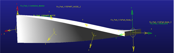
Figure 13 Twisted straight-axis beam
! Version 1
! Nodes
MATRIX/1, FULL=RORDER, ROWS=4, COLUMNS=7, VALUES =
, 10, 0.0, 0, 0, 0, 0D, 0
, 11, 1.0, 0, 0, 0, 30D, 0
, 12, 2.0, 0, 0, 0, 60D, 0
, 13, 3.0, 0, 0, 0, 90D, 0
! Section properties
MATRIX/2, FULL=RORDER, ROWS=4, COLUMNS=6, VALUES =
, 10, 0.5, 4.E+4, 1.E+2, 0, 2E+4
, 11, 0.5, 4.E+4, 1.E+2, 0, 2E+4
, 12, 0.5, 4.E+4, 1.E+2, 0, 2E+4
, 13, 0.5, 4.E+4, 1.E+2, 0, 2E+4
! Beam
FE_PART/2
, TYPE = 3DBEAM
, NODE_LABELS = 10, 11, 12, 13
, COORDINATES_MATRIX = 1
, SECTION_MATRIX = 2
, MATERIAL=1
Notice the cross sectional properties in MATRIX/2 are constant along the axis of the beam. The beam above could also be defined as follows:
! Version 2
! Nodes
MATRIX/1, FULL=RORDER, ROWS=4, COLUMNS=7, VALUES =
, 10, 0.0, 0, 0, 0, 0, 0
, 11, 1.0, 0, 0, 0, 0, 0
, 12, 2.0, 0, 0, 0, 0, 0
, 13, 3.0, 0, 0, 0, 0, 0
! Section properties
MATRIX/2, FULL=RORDER, ROWS=4, COLUMNS=6, VALUES =
, 10, 0.5, 4.E+4, 1.E+2, 0, 2E+4
, 11, 0.5, 9.E+3, 2.E+3, 2.E+1, 2E+4
, 12, 0.5, 2.E+3, 9.E+3, 2.E+1, 2E+4
, 13, 0.5, 1.E+2, 4.E+4, 0, 2E+4
! Beam
FE_PART/2
, TYPE = 3DBEAM
, NODE_LABELS = 10, 11, 12, 13
, COORDINATES_MATRIX = 1
, SECTION_MATRIX = 2
, MATERIAL=1
Notice the nodes in this second are equally oriented but the section properties change accordingly. Both versions define equivalent beam properties
3. Example
Figure 14 below shows a section of a coil to be modeled by a curved distributed-mass beam. The nodal coordinates were computed using a user-written script. The coil has constant cross section properties
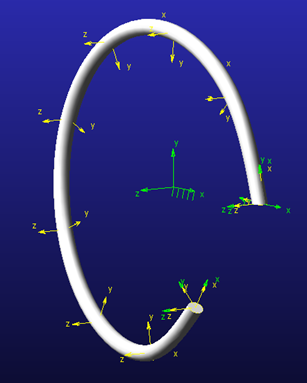
Figure 14 A coil to be modeled using a curved distributed-mass beam
! Nodes
MATRIX/11, FULL=RORDER, ROWS=9, COLUMNS=7, VALUES =
, 21, 5.0000, 0.0000, 0.0000, 0.0000, 0.0599, 1.5708
, 22, 3.8303, 3.2139, 0.2094, 0.6981, 0.0599, 1.5708
, 23, 0.8684, 4.9240, 0.4189, 1.3962, 0.0599, 1.5708
, 24, -2.4997, 4.3303, 0.6283, 2.0943, 0.0599, 1.5708
, 25, -4.6983, 1.7105, 0.8377, 2.7924, 0.0599, 1.5708
, 26, -4.6986, -1.7096, 1.0472, 3.4906, 0.0599, 1.5708
, 27, -2.5005, -4.3298, 1.2566, 4.1887, 0.0599, 1.5708
, 28, 0.8675, -4.9242, 1.4660, 4.8868, 0.0599, 1.5708
, 29, 3.8297, -3.2146, 1.6755, 5.5849, 0.0599, 1.5708
! Section properties. All nodes have the same values
MATRIX/21, FULL=RORDER, ROWS=9, COLUMNS=6, VALUES =
, 21, 0.5, 2.E+2, 2.E+2, 0, 4.E+2
, 22, 0.5, 2.E+2, 2.E+2, 0, 4.E+2
, 23, 0.5, 2.E+2, 2.E+2, 0, 4.E+2
, 24, 0.5, 2.E+2, 2.E+2, 0, 4.E+2
, 25, 0.5, 2.E+2, 2.E+2, 0, 4.E+2
, 26, 0.5, 2.E+2, 2.E+2, 0, 4.E+2
, 27, 0.5, 2.E+2, 2.E+2, 0, 4.E+2
, 28, 0.5, 2.E+2, 2.E+2, 0, 4.E+2
, 29, 0.5, 2.E+2, 2.E+2, 0, 4.E+2
! Beam
FE_PART/2
, TYPE = 3DBEAM
, NODE_LABELS = 21, 22, 23, 24, 25, 26, 27, 28, 29
, COORDINATES_MATRIX = 11
, SECTION_MATRIX = 21
, MATERIAL=1
For more information refer the FE_PART Appendix section.
FAQ
1. Why the coordinates and section properties need to have an additional column with the node number information?
One reason is that users may want to label their nodes with arbitrary numbers. Second, the user may specify a different set of nodes by simply removing/adding nodes from the NODES list. Adams Solver C++ will ignore the nodal information not set in the NODES option.
2. Can two or more FE_PART have the same node numbers?
Yes, this allows users to duplicate statements for beams. However, users will need to take care of assigning new IDs to MARKERs.
3. Can 2D beams have an offset with respect to the main global coordinate planes?
Yes, just like 2D PARTS, 2D beams may be located on a plane with an offset set by the QG option.
Limitations
Adams Solver C++ has the following limitation for FE_Part:
1. No SAVE/RELOAD support.