GSE
The GSE (General State Equation) statement lets you represent a subsystem that has well defined inputs (u), internal states (x), and a set of well defined outputs (y).
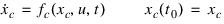
The GSE is represented mathematically as:
 | (1) |
 | (2) |
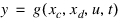 | (3) |
It consists of continuous states xc, and discrete states xd. The continuous states xc are defined in Equations (1) as explicit, first-order, ordinary differential equations. fc() is specified in a user-written subroutine, and is assumed to be continuous everywhere. Integrators in Adams Solver (FORTRAN) evaluate fc() as needed.
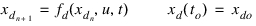
The discrete states xd are defined in Equations (2) by the function fd(). fd() is specified in a second user-written subroutine. Equations (2) are difference equations. A sampling period is associated with Equations (2), and integrators only evaluate Equations (2) at the sample times. The discrete states, xd, are assumed to be constant between sampling periods. In Equations 2, is the short form for xd(tn).
is the short form for xd(tn).The output, y, is sampled continuously, and is defined by g(). g() is specified in a third user-written subroutine. It may be discontinuous in nature. If the output is to be fed back into the mechanical system through a force element, then it is customary to eliminate the discontinuities in y, by passing it through a low-pass filter before feeding the signal into the force element. You can use the TFSISO element to define a low-pass filter. Failure to eliminate discontinuities in y will cause significant integration difficulties.
If Equations (1) are not present, the GSE is classified as a purely discrete GSE. If Equations (2) are not present, the GSE is classified as being purely continuous. If both Equations (1) and (2) are present, the GSE is classified as a sampled system. When neither Equations (1) nor (2) are present, the GSE does not contain any internal states.
Format
Arguments
FUNCTION=USER(r1[,...,r30]) | Specifies the parameters that are to be passed to the user-written subroutines that define the constitutive equations of a GSE, viz., Equations (1), (2), and (3). Three user subroutines are associated with a GSE. ■GSE_DERIV is called to evaluate fc() in Equations (1). ■GSE_UPDATE is called to evaluate fd() in Equations (2). ■GSE_OUTPUT is called to evaluate g() in Equations (3). |
IC=id | Identifies the ARRAY statement in the dataset that specifies the initial conditions for the continuous states in the system. This is an optional argument. When you use the IC argument, an ARRAY statement with this identifier must be in the dataset, it must be of the IC type, and it must have the number of elements specified in the argument NS. When you do not specify an IC array for a GSE statement, all the continuous states are initialized to zero. |
ICD=id | Identifies the ARRAY statement in the dataset that specifies the initial conditions for the discrete states in the system. This is an optional argument. When you use the ICD argument, an ARRAY statement with this identifier must be in the dataset, it must be of the IC type, and it must have the number of elements specified in the argument ND. When you do not specify an IC array for a GSE statement, all the discrete states are initialized to zero. |
INTERFACE=lib1::gse1, lib2::gse2, lib3::gse3, lib4::gse4 | Specifies an alternative library and subroutine names for the user subroutines GSE_DERIV, GSE_OUTPUT, GSE_UPDATE, GSE_SAMP respectively. The rules for the INTERFACE argument are the same as for the ROUTINE argument. Learn more about the ROUTINE Argument. |
ND=i | Specifies the number of discrete states in the GSE. Discrete states are updated by calling the function GSE_UPDATE at the sample times. ND defaults to zero when not specified. |
NO=i | A mandatory argument, NO, specifies the number of output equations (algebraic variables) that are used in the definition of Equation (3). If NO is greater than 0, you must also specify a Y array. GSE outputs are evaluated by calling the user written subroutine GSE_OUTPUT. |
NS=i | Specifies number of continuous states in the GSE and is used in the definition of Equations (1). If you do not specify NS, then the GSE is classified as being a continuous GSE. NS must be set to zero for a purely discrete GSE. The time derivatives of the continuous states of a GSE are evaluated by calling the user-written subroutine GSE_DERIV. NS defaults to zero when not specified. |
ROUTINE=lib1::gse1, lib2::gse2, lib3::gse3, lib4::gse4, lib5::gse5 | Specifies alternative library and subroutine names for the deprecated user subroutines GSESUB, GSEXX, GSEXU, GSEYX, GSEYU respectively. Learn more about the ROUTINE Argument. |
SAMPLE_OFFSET=r | Specifies the simulation time at which the sampling of the discrete states is to start. All discrete states before SAMPLE_OFFSET are defined to be at the initial condition specified. SAMPLE_OFFSET defaults to zero when not specified. |
SAMPLE_PERIOD=expression | Specifies the sampling period associated with the discrete states of a GSE. This tells Adams Solver (FORTRAN) to control its step size so that the discrete states of the GSE are updated at: last_sample_time + sample_period In cases where an expression for SAMPLE_PERIOD is difficult to write, you can specify it in a user-written subroutine GSE_SAMP(…). Adams Solver (FORTRAN) will call this function at each sample time to find out the next sample period. |
STATIC_HOLD | Indicates that the continuous GSE states are not permitted to change during static and quasi-static simulations. |
U=id | Designates the ARRAY statement in the dataset that is used to define the input variables for the GSE. The U argument is optional. When it is not present in the GSE statement, there are no system inputs. When you use the U argument an ARRAY with this identifier must be in the dataset. The number of inputs to the GSE statement is inferred from the number of VARIABLE statements in the U array. |
X=id | Designates the ARRAY statement in the dataset that is used to define the continuous states for the GSE. When you specify it, an ARRAY statement with this identifier must be in the dataset, it must be of the X type, and it may not be used in any other LSE, GSE, or TFSISO statement. If you specify SIZE on the ARRAY statement, it must have the same value as the argument NS. |
Y=id | Designates the ARRAY statement in the dataset that is used to define the outputs of the GSE. When you specify it, an ARRAY statement with this identifier must be in the dataset, it must be of the Y type, and it may not be used in any other LSE, GSE, or TFSISO statement. If you specify SIZE on the ARRAY statement, it must have the same value as the argument NO. |
XD=id | Designates the ARRAY statement in the dataset that is used to access the discrete states for the GSE. An ARRAY statement with this identifier must be in the dataset, it must be of the X type, and it may not be used in any other LSE, GSE, or TFSISO statement. If you specify SIZE on the ARRAY statement, it must have the same value as the argument ND. |
Extended Definition
The GSE (General State Equation) statement defines the equations for modeling a nonlinear, time varying, dynamic system. The statement is especially useful for importing nonlinear control laws developed manually or with an independent software package. It can also be used to define an arbitrary system of coupled differential and algebraic equations that can be expressed as:
 | (4) |
 | (5) |
 | (6) |
The GSE allows you to implement four different kinds of systems. These are:
Continuous Systems
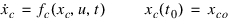
Continuous systems can be represented in the state-space form as:
 | (7) |
 | (8) |
xc is called the state of the system, and contains n elements for an nth-order system. In matrix notation, xc is a column matrix of dimension nx1. u defines the inputs to the system. Its size is equal to the number of inputs to the system being modeled. In this description, the system is assumed to have m inputs, consequently u is a column matrix of size mx1. y defines the outputs from the system. If a system has p outputs, y is represented with a column matrix of dimension px1.
Using this system description, a nonlinear, second-order differential equation, with input u, such as:
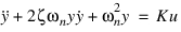 | (9) |
can be written in a state-space form as:
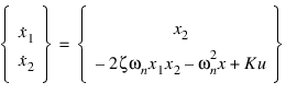 | (10) |
 | (11) |
The state Equations (7) or (10) are integrated by Adams Solver using its integrators. Therefore, it is necessary that the functional relationship expressed in Equations (7) or (10) be continuous. That is a minimum requirement for successfully integrating these equations. Similarly, if the output is to be fed back into a plant model, such as a mechanical system, Equations (8)5 or (11) are also required to be continuous. A higher degree of differentiability will help the integrators solve these equations more efficiently.
Discrete Systems
Discrete systems can be described by their difference equations. They are, therefore, represented in the state-space form as:
 | (12) |
 | (13) |
xd is called the state of the system, and contains n elements for an nth-order system. In matrix notation, xd is a column matrix of dimension nx1. u and y have the same meaning as for continuous systems.
The fundamental difference between continuous and discrete systems is that the discrete or digital system operates on samples of the sensed plant data, rather than on the continuous signal. The dynamics of the controller are represented by recursive algebraic equations, known as difference equations, that have the form shown in Equations (12).
The sampling of any signal occurs repetitively at instants in time that are T seconds apart. T is called the sampling period of the controller. In complex systems, the sampling period is not a constant, but is, instead, a function of time and the instantaneous state of the controller. The signal being sampled is usually maintained at the sampled value in between sampling instances. This is called zero-order-hold (ZOH). Determining an appropriate sampling period is a crucial design decision for discrete and sampled systems.
One major problem to avoid with sampling is aliasing. This is a phenomenon where a signal at a frequency  produces a component at a different frequency
  simply because the sampling is occurring too infrequently. The general rule of thumb for such situations is as follows:
produces a component at a different frequency simply because the sampling is occurring too infrequently. The general rule of thumb for such situations is as follows:If you want to avoid aliasing in a signal with a maximum frequency of  , the sampling frequency is calculated from
  2> 2
2> 2 . This is a lower limit for
  . If you want to obtain a reasonably smooth time response, then 20 <
  /
/ < 40.
< 40.
, the sampling frequency is calculated from 2> 2. This is a lower limit for . If you want to obtain a reasonably smooth time response, then 20 < / < 40.The sampling rate for sampling the states of a discrete system must follow the above criterion to avoid aliasing.
Note that when an Adams Solver output time and a GSE sample time coincide, the output of the GSE at that time will be calculated using the values of the discrete states before the update takes place. This is true for discrete states in discrete systems and sampled systems.
Sampled Systems
There are many systems that are neither continuous nor discrete. Some signals are sampled at discrete intervals, while others are sampled continuously. These systems are called sampled systems and are represented in the state-space for as:
 | (14) |
 | (15) |
 | (16) |
Equations (14) represent the dynamics associated with the continuous piece of the sampled system. States xc are continuous and fc() is assumed to be continuous.
Equations (15) represent the dynamics associated with the discrete piece of the sampled system. The equations are evaluated only at discrete points in time, the sample times for the sampled system. In between sample times, the discrete states are assumed to be constant.
Equation (16) defines the outputs of the system. It is important to note that the ADAMS integrators evaluate Equation (16) as often as necessary. In many problems, it is important to examine the output between sampling instants. Often, for example, the maximum overshoot may occur not at a sampling point, but between samples. This implementation allows for such observations to be made on the output.
Equation (16) defines the outputs of the system. It is important to note that the ADAMS integrators evaluate Equation (16) as often as necessary. In many problems, it is important to examine the output between sampling instants. Often, for example, the maximum overshoot may occur not at a sampling point, but between samples. This implementation allows for such observations to be made on the output.
Feed-Forward Only System
These are systems that have no independent states. The output of the system is an algebraic function of the inputs. They can be represented as:
 | (17) |
Caution: | ■The GSE statement provides a very general capability for modeling nonlinear systems. However, the routines for solving the linear equations in Adams Solver (FORTRAN) have been developed and refined to work particularly well with the sparse systems of equations that come from the assembly of mechanical models. With the GSE statement, you can create very dense sets of equations. If these equations form a large portion of the completed model, Adams Solver (FORTRAN) may perform more slowly than expected. ■During a static analysis, Adams Solver (FORTRAN) finds equilibrium values for user-defined differential variables (DIFFs, GSEs, LSEs, and TFSISOs), as well as for the displacement and force variables. This changes the initial conditions for a subsequent analysis. If STATIC_HOLD is not specified, during a static analysis, Adams Solver (FORTRAN) sets the time derivatives of the user-defined variables to zero, and uses the user-supplied initial-condition values only as an initial guess for the static solution. Generally, the final equilibrium values are not the same as the initial condition values. Adams Solver (FORTRAN) then uses the equilibrium values of the user-defined variables as the initial values for any subsequent analysis, just as with the equilibrium displacement and force values. However, the user-specified initial conditions are retained as the static equilibrium values when STATIC_HOLD is specified. Thus, the final equilibrium values are the same as the user-specified initial conditions. Note that this does not guarantee that the time derivatives of the user-defined variable are zero after static analysis. |
Examples
Modeling Continuous Control Systems
The example below demonstrates how you can use a GSE to define a continuous controller in ADAMS. The plant consists of a block on a translational joint. A continuous control force is to be applied to the block so that it translates exactly 150 mm from its initial position. The control system is defined as follows.
Inputs
■It has two inputs (u1 and u2).
■The first input (u1) is the location of the block.
■The second input (u2) is the velocity of the block.
Outputs
■It has one output, y.
■The output is an actuator signal.
States
■The controller is a linear PID controller.
■It has two continuous states (x1 and x2).
Transfer Functions
The transfer functions for the controller is:
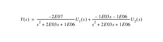
Putting the above equation in state-space representation, we obtain:
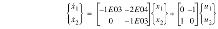
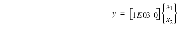
Or


In this example, a GSE will be used to define the state-space representation of the controller. Using DATA statements, matrices [A], [B] are entered in the GSE’s function GSE_DERIV, while matrix [C] is entered in the GSE’s function GSE_OUTPUT (see code below). Standard Adams modeling elements PART, JOINT, and SFORCE represent the block, translational joint, and the actuator, respectively.
Model Input File
GSE Test: Continuous states=2, Discrete states=0, Outputs=1
units/force=newton, mass=kilogram, length=millimeter, time = second
part/1, ground
marker/3, part = 1, reuler = 90d, 90d, 0d
marker/5, part = 1, qp = -150, 0, 0, reuler = 90d, 90d, 0d
part/2, qg = 0, 0, -100, mass = 46, cm = 6, ip = 2e5, 5e5, 4e5
marker/2, part = 2, qp = 0, 0, 100, reuler = 90d, 90d, 0d
marker/4, part = 2, qp = -150, 0, 100, reuler = 90d, 90d, 0d
marker/6, part = 2, qp = 0, 0, 100
marker/7, part = 2, qp = -150, 0, 100
joint/1, trans, i = 2, j = 3
sforce/1, trans, i = 4, j = 5, actiononly, function = aryval(2,1)
variable/2, function = dx(7)
variable/3, function = vx(7)
array/1, u, size = 2, variables = 2, 3 !Inputs for the GSE
array/2, y, size = 1 !Outputs for the GSE
array/3, x, size = 2 !States for the GSE
gse/99, ns = 2, no = 1, x = 3, u = 1, y = 2, function = user(3,1)
accgrav/jgrav = -9806.65
results/formatted
END
Simulation Results
The figure below shows the time history of the location and velocity of the block. Notice the displacement (red curve) starts at 0 mm, and stops moving when it reaches a value of 150 mm. Notice also the overshoot in the displacement of the block, which is subsequently corrected by the controller.
Time History of the Block Location
The next figure shows the time history of the actuator signal computed by the controller. This is the force applied on the block. Notice that the actuator signal changes sign when the block is about to overshoot its target value.
Time History of Actuator Signal Output by the Controller
User-Written Subroutines for the continuous controller modeled by GSE
SUBROUTINE GSE_DERIV(ID, TIME, PAR, NPAR, DFLAG, IFLAG, NS, XDOT)
C
C Inputs:
C
INTEGER ID, NPAR, NS
DOUBLE PRECISION PAR(*), TIME
LOGICAL IFLAG, DFLAG
C
C Outputs:
C
DOUBLE PRECISION XDOT(*)
C
C Local Variables:
C
LOGICAL LEFLAG, PARFLG
INTEGER AX(1), AU(1), NSS, NU
DOUBLE PRECISION A(2,2), B(2,2), X(2), U(2)
SAVE A, B
DATA A /-1.0e3, 0.0, -2.0e4, -1.0e3/
DATA B /0.0, 1.0, -1.0, 0.0/
C
C+--------------------------------------------------------------------*
C
C Define the function fc():
C
AX(1) = NINT(PAR(1))
AU(1) = NINT(PAR(2))
CALL SYSARY ('ARRAY', AX, 1, X, NSS, LEFLAG)
CALL SYSARY ('ARRAY', AU, 1, U, NU, LEFLAG)
XDOT(1) = A(1,1)*X(1)+A(1,2)*X(2) + B(1,1)*U(1)+B(1,2)*U(2)
XDOT(2) = A(2,1)*X(1)+A(2,2)*X(2) + B(2,1)*U(1)+B(2,2)*U(2)
C
C Return the partial derivatives to ADAMS:
C
CALL ADAMS_NEEDS_PARTIALS (PARFLG)
IF (PARFLG) THEN
CALL SYSPAR ('ARRAY', AX, 1, A, NSS*NSS, LEFLAG)
CALL SYSPAR ('ARRAY', AU, 1, B, NSS*NU , LEFLAG)
ENDIF
RETURN
END
C
C+====================================================================*
C
SUBROUTINE GSE_OUTPUT (ID, TIME, PAR, NPAR, DFLAG, IFLAG, NO, Y)
C
C Inputs:
C
INTEGER ID, NPAR, NO
DOUBLE PRECISION PAR(*), TIME
LOGICAL IFLAG, DFLAG
C
C Outputs:
C
DOUBLE PRECISION Y(NO)
C
C Local Variables:
C
LOGICAL LEFLAG, PARFLG
INTEGER AX(1), NS
DOUBLE PRECISION C(2), X(2)
SAVE C
DATA C/1.0e3, 0.0/
C
C+--------------------------------------------------------------------*
C
C Define the function g():
C
AX(1) = NINT(PAR(1))
CALL SYSARY ('ARRAY', AX, 1, X, NS, LEFLAG)
Y(1) = C(1)*X(1) + C(2)*X(2)
C
C Return the partial derivatives to ADAMS:
C
CALL ADAMS_NEEDS_PARTIALS (PARFLG)
IF (PARFLG) THEN
CALL SYSPAR ('ARRAY', AX, 1, C, NS, LEFLAG)
ENDIF
C
C
RETURN
END
Purely Discrete GSE
The example below demonstrates how you can use a GSE to define a discrete controller in ADAMS. The plant consists of a block on a translational joint. A discrete control force is applied to the block to move it exactly 150 mm from its initial position. The controller has a sample time of 0.001 seconds. The control system is defined as follows:
Inputs
■It has two inputs (u1 and u2).
■The first input (u1) is the location of the block.
■The second input (u2) is the velocity of the block.
Outputs
■It has one output, y.
■The output is an actuator signal.
States
■The controller is a linear PID controller.
■It has two discrete states (x1 and x2).
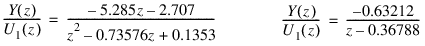
The transfer functions of the controller are:
A GSE represents the controller. Standard ADAMS modeling elements PART, JOINT, and SFORCE represent the block, translational joint, and the actuator, respectively.
GSE Test: Continuous states=0, Discrete states=2, Outputs=1
UNITS/FORCE=NEWTON, MASS=KILOGRAM, LENGTH=MILLIMETER, TIME=SECOND
PART/1, GROUND
MARKER/3, PART = 1, REULER = 90D, 90D, 0D
MARKER/5, PART = 1, QP = -150, 0, 0, REULER = 90D, 90D, 0D
PART/2, QG = 0, 0, -100, MASS = 46, CM = 6, IP =2E5, 5E5, 4E5
MARKER/2, PART = 2, QP = 0, 0, 100, REULER = 90D, 90D, 0D
MARKER/4, PART = 2, QP = -150, 0, 100, REULER = 90D, 90D, 0D
MARKER/6, PART = 2, QP = 0, 0, 100
MARKER/7, PART = 2, QP = -150, 0, 100
JOINT/1, TRANS, I = 2, J = 3
SFORCE/1, TRANS, I = 4, J = 5, ACTIONONLY, FUNCTION = ARYVAL(2,1)
VARIABLE/2, FUNCTION = DX(7)
VARIABLE/3, FUNCTION = VX(7)
ARRAY/1, U, SIZE = 2, VARIABLES = 2, 3
ARRAY/2, Y, SIZE = 1
ARRAY/3, X, SIZE = 2
GSE/99, ND=2, NO = 1, XD = 3, U = 1, Y = 2
, Sample_Period = 0.001/
, FUNCTION = USER(3,1)/
ACCGRAV/JGRAV = -9806.65
RESULTS/FORMATTED
END
Simulation Results
The figure below below shows the time history of the location and velocity of the block. Notice the displacement (red curve) starts at 0 mm, and stops moving when it reaches a value of 150 mm.
Time History of the Block Location
The next figure shows the time history of the actuator signal computed by the controller. This is the force applied on the block. Zooming into the curve shows that the output of the controller is discrete. Because the sampling period of the controller is 0.001 seconds, output was requested every 0.0005 seconds in order to see the discrete nature of the output. The states also show similar behavior.
Time History of Actuator Signal Output by the Discrete Controller
User Subroutines for the Discrete Controller Modeled by a GSE
SUBROUTINE GSE_OUTPUT (ID, TIME, PAR, NPAR, DFLAG, IFLAG, NO, Y)
C
C Inputs:
C
INTEGER ID, NPAR, NO
DOUBLE PRECISION PAR(*), TIME
LOGICAL IFLAG, DFLAG
C
C Outputs:
C
DOUBLE PRECISION Y(NO)
C
C Local Variables:
C
LOGICAL LEFLAG
INTEGER AXD(1), ND
DOUBLE PRECISION C(2), XD(2)
SAVE C
DATA C/1.0e3, 0.0/
C
C+---------------------------------------------------------------------*
C
C Y = C*Xd
C
AXD(1) = NINT(PAR(1))
CALL SYSARY ('ARRAY', AXD, 1, XD, ND, LEFLAG)
Y(1) = C(1)*XD(1) + C(2)*XD(2)
C
C
RETURN
END
C
C+====================================================================*
C
SUBROUTINE GSE_UPDATE (ID, TIME, PAR, NPAR, DFLAG, IFLAG, ND,
* XDplus1)
C
C Inputs:
C
INTEGER ID, NPAR, ND
DOUBLE PRECISION PAR(*), TIME
LOGICAL IFLAG, DFLAG
C
C Outputs:
C
DOUBLE PRECISION XDplus1(ND)
C
C Local Variables:
C
LOGICAL LEFLAG
INTEGER AXD(1), AU(1), NDD, NU
DOUBLE PRECISION A(2,2), B(2,2), XD(2), U(2)
SAVE A, B
DATA A/.36788, 0.0, -7.3576, .36788/
DATA B/-.0052848, 0.00063212, -.00063212, 0.0/
C
C+---------------------------------------------------------------------*
C
C Xd+1 = A*Xd + B*U
C
AXD(1) = NINT(PAR(1))
AU (1) = NINT(PAR(2))
CALL SYSARY ('ARRAY', AXD, 1, XD, NDD, LEFLAG)
CALL SYSARY ('ARRAY', AU , 1, U , NU, LEFLAG)
XDplus1(1) = A(1,1)*XD(1)+ A(1,2)*XD(2) + B(1,1)*U(1) + B(1,2)*U(2)
XDplus1(2) = A(2,1)*XD(1)+ A(2,2)*XD(2) + B(2,1)*U(1) + B(2,2)*U(2)
C
C
RETURN
END
C
C+====================================================================*
C
Sampled GSE
The example below demonstrates how you can use a GSE to define a sampled controller in Adams. The plant consists of a block on a translational joint. A sampled system controls the block to move it exactly 150 mm from its initial position.
The controller is modeled in Simulink. Real Time Workshop (RTW) is then employed to generate the governing equations for the GSE. An interface is then written between the code generated by RTW and the GSE subroutines: GSE_DERIV, GSE_UPDATE, GSE_OUTPUT, and GSE_SAMP.
The controller is modeled in Simulink. Real Time Workshop (RTW) is then employed to generate the governing equations for the GSE. An interface is then written between the code generated by RTW and the GSE subroutines: GSE_DERIV, GSE_UPDATE, GSE_OUTPUT, and GSE_SAMP.
The block diagram for the sampled control system is shown below:
Block Diagram of the Sampled System Used to Control the Block
The control system is defined as follows:
Inputs
■It has two inputs (in1 and in2).
■The first input (in1) is the velocity of the block.
■The second input (in2) is the location of the block.
States
■The controller has two continuous states.
■It has three discrete states.
Outputs
■It has one output, out1.
■The output is an actuator signal, which is a function of the continuous and the discrete states of the controller and the two inputs. A low pass filter, Fcn2, is employed to obtain a smooth output that may be fed into the mechanical system.
The controller is represented in a GSE. The block, translational joint, and the actuator are represented using the standard ADAMS modeling elements PART, JOINT, and SFORCE, respectively.
To see a representation of the model and a Simulink representation of the control system, see the Release Notes.
Simulation Results
The figure below shows the time history of the control force on the block. Notice that the control force changes sign when the block overshoots its desired position.
Time History of the Actuator Force on the Block
See other Generic systems modeling available.