INTEGRATOR
The INTEGRATOR statement lets you control the numerical integration of the equations of motion for a dynamic analysis. You should use the INTEGRATOR statement when the default values for the numerical solution parameters are not optimal for a particular simulation.
Format
Arguments
ABAM | Specifies that the ABAM (Adams-Bashforth-Adams-Moulton) integrator is to be used for integrating the differential equations of motion. This integrator is suitable for systems that are not stiff, that is, systems that are characterized by a undamped transients. Default: GSTIFF |
ADAPTIVITY=r | All of the BDF integrators GSTIFF, WSTIFF, and CONSTANT_BDF) use Newton-Raphson iterations to solve the nonlinear Differential-Algebraic Equations (DAE) of motion. This iteration process is referred to as correcting the solution. ADAPTIVITY modifies the corrector error tolerance to include a term that is inversely proportional to the integration step size. This is intended to loosen the corrector tolerance when the step size gets small (many corrector failures occur because of small step size). If the integration step size is equal to h, ADAPTIVITY/h is added to the corrector tolerance. When using ADAPTIVITY, begin with a small number, such as ADAPTIVITY=1E-8. Note that this relaxes the tolerance of the corrector, which can introduce additional error into the dynamic solution. The corrector tolerance must be at least a factor of 10 stricter than the integration tolerance. The ratio advocated in the theoretical literature ranges from .1 to .001 and is a function of the integrator order and step size. The ratio that Adams Solver (FORTRAN) uses varies with the integrator chosen, but is within the range specified above. If you use ADAPTIVITY to relax the corrector tolerances, be sure to validate your results by running another simulation using a different integration error tolerance. ADAPTIVITY affects only the GSTIFF, WSTIFF, and CONSTANT_BDF integrators. ADAPTIVITY is typically required to overcome corrector convergence difficulties and you should not use it in normal situations. Default: 0 Range: ADAPTIVITY > 0 |
CONSTANT_BDF | Specifies that the CONSTANT_BDF integrator is to be used for integrating the differential equations of motion. Default: GSTIFF |
 | Specifies the corrector algorithm that is to be used with the stiff integrators GSTIFF, WSTIFF, or CONSTANT_BDF. The corrector in a stiff integrator ensures that all candidate solutions satisfy the equations of the system. The two algorithms, original and modified, differ primarily in the algorithm that they use to define when the corrector iterations have converged. ■CORRECTOR=original - Specifies that the corrector available in the previous releases of Adams Solver (FORTRAN) be used. This is the default. This implementation of the corrector requires that at convergence, the error in all solution variables be less than the corrector error tolerance. ■CORRECTOR=modified - Specifies that a modified corrector is to be used. This implementation of the corrector requires that at convergence, the error in only those variables for which integration error is being monitored, be less than the corrector error tolerance. This is a slightly looser definition of convergence, and you should use proper care when using this. The CORRECTOR=modified setting is helpful for models containing discontinuities in the forcing functions. Problems with contacts belong in this category. |
ERROR=r | Specifies the relative and absolute local integration error tolerances that the integrator must satisfy at each step. For BDF integrators, Adams Solver (FORTRAN) monitors the integration errors in the displacement and state variables that the other differential equations (DIFFs, LSEs, GSEs, and TFSISOs) define. ABAM, SI1, and SI2 formulations also monitor errors in velocity variables. The larger the ERROR, the greater the error/step in your solution. Note that the value for ERROR is units-sensitive. For example, if a system is modeled in mm-kg-s units, the units of length must be in mm. Assuming that all the translational states are larger than 1mm, setting ERROR=1E-3 implies that the integrator monitors all changes of the order of 1 micron. The error tolerance is compared against a local error measure that depends on the difference between the current predicted and corrected states, the past history of the states, and the current integration order. Default: 1E-3 Range: ERROR > 0 |
GSTIFF | Specifies that the GSTIFF (Gear) integrator is to be used for integrating the differential equations of motion. |
HINIT=r | Defines the initial time step that the integrator attempts. Default: 1/20 of the output step Range: 0 < HMIN < HINIT < HMAX |
HMAX=r | Defines the maximum time step that the integrator is allowed to take. Default: When setting the argument INTERPOLATE = ON, the integration step size is limited to the value specified for HMAX, but if HMAX is not defined, no limit is placed on the integration step size. If INTERPOLATE = OFF, the maximum step size is limited to the output step. Range: 0 < HMIN < HINIT < HMAX Note: HMAX is not applicable to RKF45. |
HMIN=r | Defines the minimum time step that the integrator is allowed to take. Default: 1.0E-6*HMAX for GSTIFF and WSTIFF. Machine precision for ABAM, SI1, and the SI2 formulation Range: 0 < HMIN < HINIT < HMAX |
 | Specifies that the integrator is not required to control its step size to hit an output point. Therefore, when the integrator crosses an output point, it computes a preliminary solution by interpolating to the output point. It then refines or reconciles the solution to satisfy the equations of motion and constraint. INTERPOLATE=OFF turns off interpolation for the chosen integrator. Default: OFF for GSTIFF and WSTIFF; ON for ABAM Note: Interpolation is not supported for CONSTANT_BDF or RKF45. |
I3 | Specifies the Index-3 (I3) formulation be used. For more information, see Extended Definition. Default: I3 |
KMAX=i | Indicates the maximum order that the integrator can use. The order of integration refers to the order of the polynomials used in the solution. The integrator controls the order of the integration and the step size, and thus, controls the local integration error at each step so that it is less than the error tolerance specified. Note: For problems involving discontinuities, such as contacts, setting KMAX=2 can improve the speed of the solution. However, we do not recommend that you set the KMAX parameter unless you are a very experienced user. Any modification can adversely affect the integrators accuracy and robustness. Default: KMAX = 12 (ABAM); KMAX = 6 (GSTIFF, WSTIFF, and CONSTANT_BDF) Range: 1 < KMAX < 12 (ABAM); 1 < KMAX < 6 (GSTIFF, WSTIFF, and CONSTANT_BDF) Note: KMAX is not applicable to RKF45. |
MAXIT=i | Specifies the maximum number of iterations allowed for the Newton-Raphson iterations to converge to the solution of the nonlinear equations. The correctors in GSTIFF and WSTIFF use the Newton-Raphson iterations. ABAM also uses Newton-Raphson iterations to solve for the dependent coordinates. MAXIT should not be set larger than 10. This is because round-off errors start becoming large when a large number of iterations are taken. This can cause an error in the solution. Default: 10 Range: MAXIT > 0 |
PATTERN=c1[:...:c10] | Indicates the pattern of trues and falses for re-evaluating the Jacobian matrix for Newton-Raphson. A value of true (T) indicates that Adams Solver (FORTRAN) is evaluating a new Jacobian matrix for that iteration. A value of false (F) indicates that Adams Solver (FORTRAN) is using the previously calculated Jacobian matrix as an approximation of the current one. PATTERN accepts a sequence of at least one character string and not more than 10 character strings. Each string must be either TRUE or FALSE, which you can abbreviate with T or F. You must separate the strings with colons. Default: T:F:F:F:T:F:F:F:T:F Note: A pattern setting of all false, implies that Adams Solver (FORTRAN) is to not evaluate the Jacobian until it encounters a corrector failure. For problems that are almost linear or are linear, this setting can improve simulation speed substantially. |
RKF45 | Specifies that a Runge-Kutta-Fehlberg (4,5) method be used to integrate the differential equations governing the system being modeled. RKF45 is a single-step method unlike the BDF methods (GSTIFF, WSTIFF, or CONSTANT_BDF) or ABAM. It is primarily designed to solve non-stiff and mildly stiff differential equations when derivative evaluations are not expensive. In general, you should not use it to get highly accurate results nor answers at a great many specific points. Internally, RKF45 uses the DDERKF integrator written by L.F. Shampine and H.A. Watts. DDERKF attempts to discover when it is not suitable for the task posed. For more information, see the Extended Definition. |
SCALE=r1[,r2][,r3] | SCALE applies to only WSTIFF and ABAM. It is not applicable to GSTIFF and CONSTANT_BDF. SCALE scales the sum of the relative and absolute error tolerances. If T is the sum of the relative and absolute error tolerances applied to the state vector, then the following tolerance is applied: ■r1 * T to the translational displacements ■r2 * T to the angular displacements ■r3 * T to the modal coordinates Note: By default, error tolerance is uniformly applied to all of the displacement and angular coordinates. Default: ■WSTIFF, ABAM, and RKF45: SCALE = 1, 1, 1e-3 ■GSTIFF and CONSTANT_BDF: You cannot control SCALE Range: SCALE [i] > 0 where i = 1, 2, or 3 |
SI1 | Specifies that the Stabilized Index-1 (SI1) formulation, in conjunction with the GSTIFF, WSTIFF, or CONSTANT_BDF integrator, be used for formulating and integrating differential equations of motion. The SI1 formulation takes into account constraint derivatives when solving for equations of motion. In addition, it monitors the integration error on the impulse of the Lagrange Multipliers in the system. These additional safeguards enable the integrators to monitor the integrator error in velocity variables and the impulse of the Lagrange Multipliers. Simulations results are therefore very accurate. A positive side effect of the SI1 formulation is that the Jacobian matrix remains stable at small step sizes, which in turn increases the stability and robustness of the corrector at small step sizes. For additional information, see the Extended Definition. Default: I3 |
SI2 | Specifies that the Stabilized Index-2 (SI2) formulation, in conjunction with the GSTIFF or CONSTANT_BDF integrator, be used for formulating and integrating differential equations of motion. The SI2 formulation takes into account constraint derivatives when solving for equations of motion. This process enables the GSTIFF integrator to monitor the integration error of velocity variables, and, therefore, renders highly accurate simulations. A positive side effect of the SI2 formulation is that the Jacobian matrix remains stable at small step sizes, which in turn increases the stability and robustness of the corrector at small step sizes. The SI2 formulation is available only with GSTIFF, WSTIFF, and CONSTANT_BDF. For additional information, see the Extended Definition. Default: I3 |
WSTIFF | Specifies that the WSTIFF (Wielenga stiff) integrator be used for integrating the equations of motion. WSTIFF uses the BDF method that takes step sizes into account when calculating the coefficients for any particular integration order. Default: GSTIFF |
Extended Definition
You use the INTEGRATOR statement to select an integrator when you choose to perform a dynamic analysis. The dynamic analysis of a mechanical system consists essentially of numerically integrating the nonlinear differential equations of motion.
Ordinary differential equations (ODEs) can be characterized as being stiff or non-stiff. A set of ODEs is said to be stiff when it has widely separated eigenvalues (low and high frequencies) with the high frequency eigenvalues being overdamped. Therefore, while the system has the ability to vibrate at high frequencies, it usually does not because of the associated high damping, which dissipates this mode of motion.
The stiffness ratio of a set of ODEs is defined as the highest inactive frequency divided by the highest active frequency. Stiff ODEs typically have a stiffness ratio of 200 or higher. In contrast, non-stiff systems have a stiffness ratio less than 20. This basically means that for a non-stiff system of ODEs, the higher frequencies of the system are active. The system can and does vibrate at these frequencies.
An example of a stiff system is a flexible body in which the higher frequencies have been damped out completely, leaving only the lower frequency vibration modes active.
The system above becomes non-stiff if the higher frequencies are excited by an external force. Nonlinear ODEs can be stiff at some points in time and non-stiff at other points.
Stiff and Non-Stiff Integrators
Integrators are classified as stiff or non-stiff. A stiff integrator is one that can handle numerically stiff systems efficiently. For stiff integrators, the integration step is limited by the inverse of the highest active frequency in the system. For non-stiff integrators, the integration step is limited by the inverse of the highest frequency (active or inactive) in the system. Thus, non-stiff integrators are notoriously inefficient for solving stiff problems.
Because many mechanical systems are numerically stiff, the default integrator in Adams Solver (C++) is GSTIFF, a stiff integrator that is based on the DIFSUB integrator developed by C.W. Gear. The DIFSUB integrator by C.W. Gear is unrelated to the Adams Solver subroutine that is known by the same acronym. Adams Solver (FORTRAN) also provides two additional stiff integrators: CONSTANT_BDF and WSTIFF. All of these integrators are based on Backward-Difference Formulae (BDF) and are multi-step integrators. The solution for these integrators occurs in two phases: a Prediction followed by a Correction.
Note: |
Prediction
When taking a new step, the integrator fits a polynomial of a given order through the past values of each system state, and then extrapolates them to the current time to perform a prediction. Standard techniques like Taylor's series (GSTIFF) or Newton Divided Differences (WSTIFF) are used to perform the prediction.
Prediction is an explicit process in which only past values are considered, and is based on the premise that past values are a good indicator of the current values being computed. The predicted value does not guarantee that it will satisfy the equations of motion or constraint. It is simply an initial guess for starting the correction, which ensures that the governing equations are satisfied.
The degree of polynomial used for prediction is called the order of the predictor. For example, a predictor of order 3 will fit a cubic polynomial that includes the past 4 values for each state. Clearly, if the governing equations are smooth, the prediction will be quite accurate. On the other hand, if the governing equations are not smooth, the prediction can be quite inaccurate.
Correction
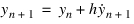
The corrector formulae are an implicit set of difference relationships (BDFs) that relate the derivative of the states at the current time to the values of the states themselves. This relationship transforms the nonlinear differential algebraic equations to a set of nonlinear, algebraic difference equations in the system states. The Backward Euler integrator is an example of a first-order BDF. Given a set of ODEs of the form dy/dt = f (y,t), the Backward Euler uses the difference relationship:
 | (18) |
where:
■yn is the solution calculated at t = tn.
■h is the step size being attempted.
■yn+1 is the solution at = tn+1, which is being computed.
Notice that the subscript n+1 is on both sides of Equation (18). This is an implicit method.
Adams Solver (FORTRAN) uses an iterative, quasi-Newton-Raphson algorithm to solve the difference equations and obtain the values of the state variables. This algorithm ensures that the system states satisfy the equations of motion and constraint. The Newton-Raphson iterations require a matrix of the partial derivatives of the equations being solved with respect to the solution variables. This matrix, known as the Jacobian matrix, is used at each iteration to calculate the corrections to the states.
Assume that the equations of motion have the form:
 | (19) |
where y represents all the states of the system.
 and
and  gives:
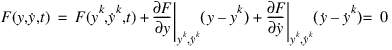
replacing y - yk with  and
and  with
with  , you get:
and with , you get: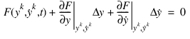 | (20) |
From Equation (18), which is a first-order BDF, you can get the relationship:
 | (21) |
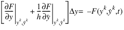 | (22) |
A generalization of (22)to higher-order BDFs gives:
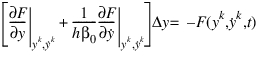 | (23) |
where:
■ scalar that is characteristic to an integration order. For each integration order this scalar is constant.
scalar that is characteristic to an integration order. For each integration order this scalar is constant. ■The matrix on the left side of Equation (23) is the Jacobian matrix of F.
■ are the corrections.
are the corrections. ■F is the residue of equations (equation imbalances).
The corrector is said to have converged when the residue F and the corrections  have become small.
have become small.After the corrector has converged to a solution, the integrator estimates the local integration error in the solution. This is usually a function of the difference between the predicted value and the corrected value, the step size, and the order of the integrator. If the estimated error is greater than the specified integration ERROR, the integrator rejects the solution and takes a smaller time step. If the estimated error is less than the specified local integration ERROR, the integrator accepts the solution and takes a new time step. The integrator repeats the prediction-correction-error estimation process until it reaches the time specified in the SIMULATE command.
Note: | The premise for using predictions as an initial guess for the corrector is severely violated when discontinuities occur or when large forces turn on or off in the model. Contact, friction, and state transitions (as in hydraulics where a valve is suddenly closed or opened) are examples of such phenomena. These kinds of models are difficult for multi-step integrators. |
GSTIFF
GSTIFF is based on the DIFSUB integrator. GSTIFF is the most widely-used and tested integrator in Adams Solver (FORTRAN). It is a variable-order, variable-step and multi-step integrator with a maximum integration order of six. The BDF coefficients it uses are calculated by assuming that the step size of the model is mostly constant. Thus, when the step size changes in this integrator, a small error is introduced in the solution. This formulation offers the following benefits and limitations:
Characteristics of GSTIFF Integrator
Benefits: | Limitations: |
|---|---|
■High speed. ■High accuracy of the system displacements. ■Robust in handling a variety of analysis problems. | ■Velocities and especially accelerations can have errors. An easy way to minimize these errors is to control HMAX so that the integrator runs at a constant step size and runs consistently at a high order (three or more). ■You can encounter corrector failures at small step sizes. These occur because the Jacobian matrix is a function of the inverse of the step size and becomes ill-conditioned at small steps. |
References
For more information on the GSTIFF integrator, see:
■Gear, C.W. (1971a). The Simultaneous Solution of Differential Algebraic Systems. IEEE Transactions on Circuit Theory,
CT-18, No.1, 89-95.
CT-18, No.1, 89-95.
■Gear, C.W. (1971b). Numerical Initial Value Problems in Ordinary Differential Equations. New Jersey: Prentice-Hall.
CONSTANT_BDF
CONSTANT_BDF is a modification of the DIFSUB integrator, to make it behave like a stable, fixed-step integrator. It is a variable-order, predominantly fixed-step, multi-step integrator, with a maximum order of six. Because it is a BDF method, it is stiffly stable, that is, it can solve stiff problems efficiently without becoming unstable.
The maximum integrator step size, HMAX, controls the integration error in CONSTANT_BDF. CONSTANT_BDF does not attempt to calculate the local integration error. If the corrector has converged, CONSTANT_BDF assumes that the solution is correct. The step size is fixed at HMAX. The integrator order is gradually increased up to KMAX. In this regard, it is very much like a fixed-step integrator.
If the corrector fails to converge, CONSTANT_BDF reduces the step size until the corrector converges. CONSTANT_BDF restores the step size to HMAX every 25 steps. CONSTANT_BDF works with both the Index-3 (I3) and the Stabilized Index-2 (SI2) formulations. We recommend that you use the SI2 formulation wherever possible because it is much more stable. Like GSTIFF, CONSTANT_BDF also works with the modified corrector, which can handle discontinuities much more effectively. To use the modified corrector, choose corrector=modified in the INTEGRATOR statement.
Unlike GSTIFF or WSTIFF, CONSTANT_BDF tends to run at the maximum allowable KMAX. A high integration order implies greater accuracy. Coupled with explicit step size control, the use of a high integrator order normally results in quite accurate solutions. If your answers do not seem to be accurate, decrease HMAX. This will give you better answers. We recommend that you scale down HMAX gradually in factors of two, because simulation times can increase when you reduce HMAX.
All integration control parameters available for GSTIFF are also available for CONSTANT_BDF.
The table below summarizes the benefits and limitations of the CONSTANT_BDF integrator.
Characteristics of CONSTANT_BDF Integrator
Benefits: | Limitations: |
|---|---|
Is very robust and stable at small step sizes when used with the SI2 formulation. | Not as fast as GSTIFF or WSTIFF for many simulations. |
Can solve problems where GSTIFF might fail. | Too large of a value for HMAX results in inaccurate answers. |
Is not as susceptible to spikes in accelerations and forces as GSTIFF. | Too small of a value for HMAX results in slow simulations. |
High accuracy in system displacements and velocities. | 000 |
SI2
SI2 (Stabilized-Index Two) is an equation formulation technique that can be used for equations describing mechanical systems. Currently, this formulation is available only with GSTIFF, WSTIFF, and CONSTANT_BDF.
To understand what the SI2 formulation does, you need to know what Differential Algebraic Equations (DAE) are and understand the notions of Index of a DAE and stabilization of DAE. A brief summary is given below. For more information, refer to:
■Brenan, K.E., Campbell, S.I., and Perzold, L.R. (1996). Numerical Solution of Initial Value Problems in Differential-Algebraic Equations, Classics in Applied Mathematics.
ISBN: 0-89871-353-6 (pbk.)
ISBN: 0-89871-353-6 (pbk.)
ODEs Versus DAEs
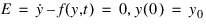 | (24) |
is defined to be a set of ODEs, because are explicit in Equation (24).
are explicit in Equation (24).Notice that for ODEs, , and is never singular.
, and is never singular.In contrast, DAEs are usually written as:
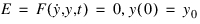 | (25) |
It is an intrinsic property of DAE that the matrix is singular. Another way of stating this is that some of the equations in a set of DAEs are not differential equations at all, they are algebraic equations of constraint.
is singular. Another way of stating this is that some of the equations in a set of DAEs are not differential equations at all, they are algebraic equations of constraint.In Adams Solver (C++), the equations of a mechanical system are formulated as:
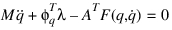 | (26) |
 | (27) |
where:
■M is the mass matrix of the system.
■q is the set of coordinates used to represent displacements.
■ is the set of configuration and applied motion constraints.
is the set of configuration and applied motion constraints. ■F is the set of applied forces and gyroscopic terms of the inertia forces.
■AT is the matrix that projects the applied forces in the direction q.
■ is the gradient of the constraints at any given state and can be thought of as the normal to the constraint surface in configuration space.
is the gradient of the constraints at any given state and can be thought of as the normal to the constraint surface in configuration space. Notice that Equation (26) is a second-order differential equation but Equation (27) is an algebraic equation. Also notice the time derivatives of q are seen in Equations (26), but  is not present in either Equation (26) or (27).
These are typical characteristics of DAEs.
is not present in either Equation (26) or (27).These are typical characteristics of DAEs.
Index of a DAE
The index of a DAE is defined as the number of time derivatives required to convert a set of DAEs to Odes
Equations (26) can be converted to a set of ODE by first taking two time derivatives of the kinematic position constraint equations in Eq.(27), to obtain the set of kinematic acceleration constraint equations. These equations together with the equations of motion in Eq.(26) can be formally solved for the accelerations and the Lagrange multipliers  . By taking a third and last time derivative of the Lagrange multipliers, one is left with a set of ODE in accelerations and the Lagrange multipliers.
. By taking a third and last time derivative of the Lagrange multipliers, one is left with a set of ODE in accelerations and the Lagrange multipliers.Therefore, the Euler-Lagrange equations for mechanical systems are said to have an Index=3.
Solution of DAEs
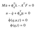
Equations (26) are converted to first-order form, so that commercially available DAE integrators can solve them. This is usually done by introducing a new variable, the velocity variable u, which is defined as:
 | (28) |
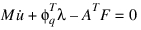 | (29) |
 | (30) |
 | (31) |
These are the DAE (in first order form) for a mechanical system. Applying the BDF formula (like Equation (21)), one obtains the Jacobian of Equation (29):
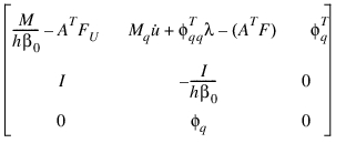
This matrix becomes ill conditioned as the integration step size h decreases, and becomes singular as h moves closer to 0.
This is the reason why Index 3 formulations become unstable at small step sizes -- a very counter-intuitive result.
Another important result for Index 3 formulations is that the integration error cannot be monitored on either velocities, u, or reaction forces, .
.
.Index reduction methods (IRM) are typically employed to make DAE more easily solvable by numerical methods. The key benefit to using IRM is that the integration error can be monitored on velocities.
Index Reduction Methods
There are many ways to reduce the index of a DAE. In general, the lower the index of a DAE, the more theoretically tractable it is to being numerically solved. So in general, it is a good idea to try to reduce the index of a DAE.
One common approach is to replace Equation (31) with the time derivatives of the constraint. Every level of differentiation reduces the index by one.
For example, you might be tempted to reduce the Index of Equation (29) to two by differentiating (31):
 | (32) |
Solving Equations (32) numerically adds a new complication, however. The solution satisfies Equation (32), but is not guaranteed to solve Equation (29), the original constraint.
If you were to formulate a simple pendulum using Equations (32) and solve them, you would notice that after some time the pin-joint constraint is violated and the pendulum drifts off into space, grossly violating the pin-joint, and the system Equation (32) is not aware.
Clearly, a means for considering Equation (31) along with Equations (32) to prevent drift-off is required. The SI2 formulation does precisely this.
The SI2 Formulation
Gear, Gupta, and Leimkuhler have shown that drift-off can be prevented by appending Equation (29) to (32) and adding a new set of variable as follows:
 | (33) |
The numerical solution of Equations (33) are guaranteed to satisfy both  and
and  . In this sense, the Equations (33) are stabilized. Because the constraints
  have been differentiated once, Equation (33) has an Index = 2.
and . In this sense, the Equations (33) are stabilized. Because the constraints have been differentiated once, Equation (33) has an Index = 2.Equations (33) are called the Stabilized Index Two representation of Equations (30). It has been proven rigorously that Equation (33) and Equation (30) have the same solution when  = 0. This condition is rigorously enforced by the SI2 formulation in Adams Solver (FORTRAN).
= 0. This condition is rigorously enforced by the SI2 formulation in Adams Solver (FORTRAN).It can also be shown that the Jacobian of Equation (33) does not become ill-conditioned as h moves closer to 0. Furthermore, since Equation (33) has an Index of 2, the integrators can monitor integration error on both u and q.
You can then, in principle, append the second time derivative of the constraints,  to Equation (33) and introduce yet another set of variables
  to reduce the index of Equations (33) to one (SI1). We have found this to be computationally very expensive and not much more accurate than the SI2 formulation.
to Equation (33) and introduce yet another set of variables to reduce the index of Equations (33) to one (SI1). We have found this to be computationally very expensive and not much more accurate than the SI2 formulation.There is, however, an alternative method for implementing the SI1 formulation that is promising.
Benefits and Limitations
The benefits and limitations of the S12 formulation are described in the following table:
Characteristics of the SI2 Formulation
Benefits of the SI2 formulation: | Limitations of the SI2 formulation: |
|---|---|
■Gives very accurate results, especially for velocities and accelerations. ■Usually allows an ERROR that is approximately 10 to 100 times larger than regular GSTIFF to produce the same quality of results. ■Is very robust and stable at small step sizes. ■Corrector failures that small step sizes cause occur less frequently than with the Index-3 GSTIFF formulation. ■Singular matrices due to small step sizes occur less frequently than with the Index-3 GSTIFF formulation. ■Corrector failures are typically indicative of a modeling problem and not of a numerical deficiency in the Adams Solver software. ■Tracks high frequency oscillations very accurately. | ■Is typically 25% to 100% slower for most problems than regular GSTIFF, when run with the same error. ■Requires that all velocity inputs be differentiable. Therefore, you must define your MOTIONS so that they are smooth and twice differentiable. Non-smooth motions, which theoretically cause infinite accelerations, cause failures in the SI2 formulation. The I3 formulations can sometimes handle such models. ■Displacement MOTIONS cannot be functions of VARIABLES. When Adams Solver encounters models containing such MOTIONS, it automatically switches to the SI3 formulation (velocity- and acceleration-based motions can be functions of VARIABLES). |
SI1 Formulation
The version of SI1 implemented in Adams Solver does not use the second-time derivative of the constraints,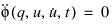 , because this is computationally very expensive.
, because this is computationally very expensive.Instead, it uses a change of variables to reduce the index. The Lagrange Multipliers  and
and  in Equations (33) are replaced by new variables
and in Equations (33) are replaced by new variables  and
and  . Therefore, Equations
 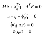 | (34) |
This change of variables has effectively reduced the index of Equations (34) to 1. This is because we only need to differentiate the velocity constraint equation once to explicitly calculate expressions for  and
and  .
.
and .Using the SI1 formulation, you can now monitor the integration error in  and
and  .
.  and
and  are defined as the impulse associated with
  and
and  , respectively. That is:
and . and are defined as the impulse associated with and , respectively. That is: | (35) |

Therefore, in the SI1 formulation, the integration error can be monitored on all states (q, u,  , and
, and  ).
).
, and ).In this respect, the SI1 formulation is even more accurate than the SI2 formulation.
In practice, we have observed that, for most models, SI1 and SI2 give the same quality of answers. However, system accelerations (that is  ) tend to be more accurate with the SI1 formulation. The performance of the SI1 formulation is also quite comparable to the SI2 formulation for many classes of models. The SI1 formulation is more sensitive and finicky for models containing significant contact or friction.
) tend to be more accurate with the SI1 formulation. The performance of the SI1 formulation is also quite comparable to the SI2 formulation for many classes of models. The SI1 formulation is more sensitive and finicky for models containing significant contact or friction.References
For more information on the SI1 and SI2 formulations, see:
■Brenan, K.E., Campbell, S.L, & Petzold, L.R. (1996). Numerical Solution of Initial-Value Problems in Differential-Algebraic Equations (Classics in Applied Mathematics, 14). Society for Industrial & Applied Mathematics; ISBN: 0898713536 (pbk).
■Gear, C.W., Leimkuhler, B., Gupta, G.K. Automatic Integration of Euler-Lagrange Equations with Constaints. Journal of Computation and Applied Mathematics, 12 & 13, pp. 79-90, North-Holland: 1985.
■Orlandea, N.V. A study of the effects of the lower index methods on ADAMS sparse tableau formulation for the computational dynamics of multi-body mechanical systems, IMechE Proc Instn Mech Engrs V01 213 Part K: 1999 1-9
WSTIFF
WSTIFF is a stiffly stable, BDF-based, variable-order, variable-step, multi-step integrator. It has a maximum order of six. The BDF coefficients it uses are a function of the integrator step size. Thus, when the step size changes in this integrator, the BDF coefficients change. WSTIFF can change step size without any loss of accuracy, which helps problems run more smoothly. The benefits and limitations of WSTIFF are the same as those of GSTIFF and are listed in the Characteristics of GSTIFF Integrator table.
References
For information on the WSTIFF integrator, see the paper:
■Van Bokhoven, W.M.G. (1975, February). Linear Implicit Differentiation Formulas of Variable Step and Order. IEEE Transactions on Circuits and Systems, 22 (2).
ABAM
ABAM (Adams Bashforth-Adams Moulton) is a non-stiff integrator based on a code originally written by Laurence F. Shampine and Marilyn K. Gordon.
ABAM is a multi-step, variable-order, variable-step integrator that has a maximum order of 12. ABAM uses a PECE (Predict-Evaluate-Correct-Evaluate) scheme to integrate a set of ordinary differential equations. ABAM may be better for simulating systems that undergo sudden changes (non-stiff systems) or for those with active, high frequencies. The easiest way to know that your system is not numerically stiff is to check that its high frequencies are underdamped. If they are, you can select ABAM. The command LINEAR/EIGEN calculates the eigenvalues for any system at a given configuration.
ABAM is a multi-step, variable-order, variable-step integrator that has a maximum order of 12. ABAM uses a PECE (Predict-Evaluate-Correct-Evaluate) scheme to integrate a set of ordinary differential equations. ABAM may be better for simulating systems that undergo sudden changes (non-stiff systems) or for those with active, high frequencies. The easiest way to know that your system is not numerically stiff is to check that its high frequencies are underdamped. If they are, you can select ABAM. The command LINEAR/EIGEN calculates the eigenvalues for any system at a given configuration.
ABAM uses coordinate partitioning, which is a method of eliminating constraint equations, such as the ones induced by joints, from the equations of motion. This method reduces the entire system of differential algebraic equations (DAEs) to a condensed set of ordinary differential equations (ODEs). It does so by selecting the coordinates (degrees of freedom) that will change the most during the simulation as the independent coordinates. Only these coordinates are integrated. All other dependent coordinates in the system can be expressed as algebraic functions of the independent coordinates through the constraints. After each successful integration step, the coordinate-partitioning algorithm computes the dependent displacements, their time derivatives, and the accelerations and Lagrange multipliers (constraint reactions). During this process, Adams Solver (FORTRAN) holds the independent coordinates constant and employs a Newton-Raphson iteration scheme to find the dependent coordinates. After computing the dependent velocities from the independent values, Adams Solver (FORTRAN) uses the Newton-Raphson algorithm again to find the full set of accelerations and Lagrange multipliers (constraint forces).
The displacement solution for the full set of dependent and independent coordinates provides the appropriate matrix for Adams Solver (FORTRAN) to explicitly solve for the velocities of the dependent coordinates. When the integrator has a complete set of displacements, velocities, accelerations, and Lagrange multipliers, it is ready to begin the next integration step.
GSTIFF, WSTIFF, and CONSTANT_BDF control only errors in displacements and user-defined variables that are specified in differential equations. This solution method is guaranteed to satisfy the equations of constraint and the equations of motion. It is not guaranteed to satisfy the first and second time derivatives of the constraint equations. This solution method usually leads to acceptable accuracy in the velocity, acceleration, and force results. However, you may find cases when the velocity, acceleration, or force results are not acceptable, even when ERROR is set appropriately and the displacement results are accurate. In these cases, you may improve accuracy by using the HMAX argument, which lets you directly limit the size of the integration steps.
The SI2 formulation and ABAM control errors in all displacements, velocities, and user-defined variables that are specified in differential equations. This solution method is guaranteed to satisfy the equations of motion, and the equations of constraint and their first time derivative. ABAM also satisfies the second time derivative of the equations of motion. This leads to increased accuracy in the velocity, acceleration, and force results, but can slow down the simulation.
Caution: | The ABAM integrator does not support the VELOCITY and ACCELERATION arguments on the MOTION statement. |
References
For more information on the methods used in the ABAM integrator, see:
■Shampine, L.F., Gordon, M.K. (1974). Computer Solutions of Ordinary Differential Equations. W. H. Freeman and Co.
For more information on coordinate partitioning and projection methods in general, see:
■Wehage, R.A. and Haug, E.J. (1982). Generalized Coordinate Partitioning for Dimension Reduction in Analysis of Constrained Dynamic Systems. Journal of Mechanical Design, Vol. 104. No. 1,247 - 255.
RKF45
RKF45 (Runge-Kutta-Fehlberg 4-5) is a single-step integrator that is based on DDERKF, originally implemented by Lawrence F. Shampine and H.A. Watts.
The Runge-Kutta-Fehlberg (RKF) methods are an extension of the traditional Runge-Kutta (RK) methods. The innovation of the RKF methods is that the local truncation error per step is computed by comparing the calculated answer yn+1 (at t = tn+1) with the result of an associated higher-order RK formula.
The Runge-Kutta-Fehlberg (RKF) methods are an extension of the traditional Runge-Kutta (RK) methods. The innovation of the RKF methods is that the local truncation error per step is computed by comparing the calculated answer yn+1 (at t = tn+1) with the result of an associated higher-order RK formula.
Therefore, in a 4-5 method, the error in the fourth-order RK method is estimated by subtracting it from the value obtained by a fifth-order RK method.
The method may be briefly summarized as follows:
Assume that we are trying to solve the differential equations:
Assume that we are trying to solve the differential equations:
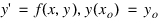 | (36) |
 | (37) |
■ be the solution at
be the solution at ■ be the integration step_size
be the integration step_size Now define:
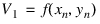
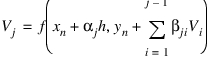
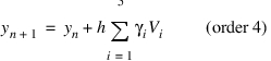
The fourth and fifth-order formulas are, respectivly:
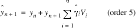
The truncation error in  is approximated by:
is approximated by: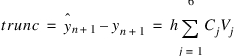
The coefficients 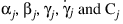 are property of the method and are known as prion.
are property of the method and are known as prion.RKF45 is primarily designed to solve non-stiff and mildly stiff differential equations, where the derivative evaluations are not expensive (time consuming). In the formulation used in Adams Solver, the derivative evaluation is expensive. Consequently, RKF45 is usually not very fast. In our testing, RKF45 is about five times slower than ABAM for most models. RKF45 is a good addition to the suite of integrators in Adams, because, unlike all the others, it is a single-step integrator, and therefore, fundamentally different.
RKF45 can only handle ordinary differential equations (ODE), and not DAE. Therefore, the DAE corresponding to the model needs to be transformed to ODE.
Like ABAM, RKF45 uses coordinate partitioning to convert the DAE into ODE. For more information about coordinate partitioning, see the third paragraph in the description of ABAM above.
References
For more information on the implementation of RKF45, see:
■SAND-79-2374, DEPAC - Design of a User Oriented Package of ODE Solvers, H.A. Watts and L.F. Shampine, Sandia Laboratories, Albuquerque, New Mexico.
Error in Handling Simulations
The following sections include descriptions and work-arounds for common error conditions you might encounter during a simulation. The sections include:
Integration Failures
An integration failure is the condition when the integrator calculates a solution, but then rejects it because it does not meet the accuracy requirements you specified. Because all integrators attempt to take the largest time step possible, failure is a fairly routine occurrence and is not cause for concern. Integrators can automatically decrease the step size and/or integrator order and repeat the step. Integration failures in multi-step methods are caused when the predictor and corrector give different answers. Such a situation can occur often when a force is suddenly turned on or off, thus, causing a discontinuity in the solution. For this reason, past values are not a good indicator of current values. The following tips can help you avoid integration failure:
■When modeling, be sure that all motion inputs, user-defined forces, and user-written differential equations are both continuous and differentiable. The smoother a function is, the easier it is to integrate. Always use a STEP or STEP5 function to switch a signal on or off, instead of using IF logic.
■Remember that cubic SPLINEs can only guarantee first-order differentiability. Inputting a SPLINE through a displacement-based MOTION causes accelerations to be spiky. Therefore, input the SPLINE in a velocity-based MOTION.
■For greater simulation control, use HMAX to control the maximum step size that the integrator can take. HMAX enables the integrator to reach higher orders and maintain them consistently.
■Be careful when using non-differentiable intrinsic functions, such as IF, MIN, MAX, SIGN, MOD, and DIM. These functions can give discontinuous answers and can cause integrator problems. The integration failure diagnostic identifies the variable and its parent modeling element with the most error in it. Examine the entities that connect to the parent modeling element to see if you can identify the cause of the failure.
Corrector Failures
A corrector failure occurs when the Newton-Raphson iterations in the correction phase do not converge to a solution. Corrector failure occurs if the predictor cannot provide a reasonable initial guess and the equations themselves are not smooth, as the Newton-Raphson algorithm assumes. A corrector failure is a fairly severe event that you should avoid by changing your model. Some tips to help avoid corrector failure are:
■As with preventing integrator failures, be sure that all motion inputs, user-defined forces, user-written differential equations, and user-defined algebraic variables are both continuous and differentiable. The smoother a function is, the easier it is to solve for it. Use a STEP or STEP5 function to switch a signal on or off instead of using IF logic.
■Use the ERROR keyword to loosen the integration error. Loosening the value for ERROR also decreases the tolerance that the corrector is required to meet.
■Use the SI2 formulation and see if the failures go away.
■Use the new corrector. Set the environment variable MDI_ADAMS_NEWCOR to TRUE and re-run your simulations.
■As a last resort, use the ADAPTIVITY keyword to force the system to loosen its corrector-error tolerance.
■Here are some diagnostic techniques for identifying the cause of some failures:
■Examine the EPRINT output from DEBUG to identify the modeling entities that are having the greatest difficulty converging.
■If the modeling element is a force:
■Make sure that the force law it obeys is smooth.
■Examine the stiffness of the force entity. Reduce it if necessary to overcome the failures.
■Examine the damping of the force entity. Damping is usually less than 5% of the stiffness. Large values of damping can also cause failures.
■If the modeling element causing the corrector failures is an equation of force/torque balance for a PART, POINT_MASS, or FLEX_BODY, try to identify the entities that may be applying anomalous forces on the body.
Look at the accelerations of the body. A large acceleration in a certain direction is always caused by a large force in that direction. Try to identify the modeling element that is causing the large acceleration, examine how it is defined, and try to understand why it is applying a large force.
Look at the accelerations of the body. A large acceleration in a certain direction is always caused by a large force in that direction. Try to identify the modeling element that is causing the large acceleration, examine how it is defined, and try to understand why it is applying a large force.
■If the modeling element is a CONTACT, review the stiffness, damping, and frictional properties of the contact. Reducing stiffness and damping helps. Similarly, increasing stiction and dynamic friction transition velocities can help the integrator.
■If the modeling element is a FRICTION entity, increasing the stiction and dynamic friction transition velocities usually helps. Evaluate the effect of reducing the friction coefficients and the pre-load.
■If the modeling element is a DIFF or GSE, make sure that the derivatives you are defining have reasonable values. Large derivatives cause problems. Make sure that the constitutive equations are smooth (differentiable) and that they do not have any kinks.
■If the modeling element is a redundant constraint, this implies that Adams Solver is having difficulty satisfying the constraint. The most likely cause for such a failure is an inconsistently defined or ill-behaved model. Eliminate the inconsistency.
■If the modeling element is a constraint reaction, try to identify the applied force or torque that is trying to break the constraint.
Integration Restarts
An integration restart is when the integrator fails to take a new step successfully. Adams Solver (FORTRAN) calculates a new and consistent set of initial conditions at the point of failure and the solution progresses with this new set of initial conditions. A restart occurs if the integrator encounters several consecutive integration failures and/or corrector failures while attempting a new step. Integration restart is usually indicative of discontinuous equations describing the system. To help avoid integration restart, you can:
■Increase ERROR value. Integration restarts sometimes occur simply because the value specified for ERROR is too small.
■Identify modeling problems in your system. Typically, a single modeling element dominates an integrator or corrector error. Identify that element and see why it may be causing problems. Smoothen its definition if there is a function expression or user subroutine associated with it. For more information on how to diagnose modeling problems, see Corrector Failures.
■Use the CONSTANT_BDF integrator, and see if the problem goes away. Step size change can destabilize correctors that assume predominantly fixed step sizes, by introducing a small error in the solution when the step size changes.
Singular Matrices and Symbolic Refactorization
A singular matrix condition occurs when the Jacobian matrix is not invertible. Recall that the corrector needs to invert the Jacobian matrix during its iterations to solve a set of linearized algebraic equations. (See Correction). A scalar analogy to a singular matrix is a divide-by-zero situation. Adams Solver (FORTRAN) does not actually invert the matrix, but calculates the matrixes Lower and Upper triangular factors (LU factors). This method of computation is very efficient and is equivalent to an inversion.
Given a Jacobian matrix, Adams Solver (FORTRAN) calculates and stores the LU factors in a symbolic form. In other words, Adams Solver (FORTRAN) explicitly calculates the LU factors as a function of the values in the Jacobian matrix. Adams Solver (FORTRAN) also assumes that the pivots are never zero. (Pivots are chosen during the Gaussian elimination and are used to factorize the matrix.) Because the equations being solved are nonlinear, it is likely that a set of pivots chosen earlier may not be optimal. Some of the pivots may become small or even zero. This event is known as the singular matrix condition. When Adams Solver (FORTRAN) encounters this condition, it recalculates the symbolic LU factors for the Jacobian matrix using the current values of the state variables. This process is known as symbolic refactorization.
Occasional occurrences with singular matrixes and symbolic refactorization are normal and are no cause for alarm. However, if these events occur frequently, you should examine your model. The typical causes for singular matrices are:
■A mass or inertia component is not specified.
■The system has reached a locked configuration, that is, it can no longer move without violating one of its constraints.
■A large force or moment has been suddenly turned on or off.
■The integrator is forced to take an extremely small step because of a hidden discontinuity in an element described in a user-written subroutine. IF statements, as well as non-differentiable intrinsic functions, such as SIGN, MOD, MIN, MAX, and so on, can create non-differentiable or even discontinuous descriptions of modeling elements. Be very careful when using these aspects of a programming language.
Common causes for singular matrices or symbolic refactorization are:
■Large force suddenly turns on. The large force is usually associated with a high stiffness. A large stiffness causes the Jacobian to become ill-conditioned.
■Your mechanical system may be in a lockup or bifurcation configuration.
■The integrator step size is too small for the I3 formulation. Switch to the SI2 formulation if you notice this.
The Index-3 Jacobian matrix (see Equation 6) contains some terms that are inversely proportional to the step size being taken. As the step size shrinks, these terms grow large. In fact, they grow so large that they eclipse all other entries in the matrix. Computers typically have difficulty dealing with matrices that have entries spanning a large range. The smaller numbers consequently get lost in round-off error, and, thus, cause singular or ill-conditioned matrices to occur. The root cause for these problems is that the step size is very small. The solution is to understand why the step size is so small, and modify the model accordingly. Discontinuities are prime causes for problems related to small steps sizes. Eliminating the discontinuities causes the integrator to take larger steps, and, therefore, avoid fatal singular matrix condition. Using the SI2 formulation can also help solve this problem.
Choosing and Integration Error
The integration ERROR is a key parameter that you need to specify for a simulation. The following are three options for calculating a reasonable value for ERROR:
For I3 formulation with GSTIFF and WSTIFF:
ERROR = VEPS *(6*Nb + 3*Np + Nu + 2*Nm)
For SI2 formulation with GSTIFF:
ERROR= K * VEPS * (12*Nb + 6*Np + Nu + 2*Nm)
For ABAM:
ERROR= K * VEPS *(2*Ndof+Nu)
where:
■VEPS is the desired error per variable per integration step.
■Nb is the number of rigid bodies in the model (excluding GROUND).
■Np is the number of point masses in the system.
■Nu is the number of user-defined differential equations in the system (DIFFs+LSEs+GSEs).
■Nm is the total number of modal coordinates in the system:
■K =10 (for smooth problems).
■K =100 (for impact and friction problems).
■Ndof = total number of mechanical degrees of freedom.
All integrators require that you input a value, referred to as ERROR in this guide, that specifies the degree of accuracy you want to achieve in a simulation. ERROR is the maximum error allowed per integration step for the entire system. This can be confusing in Adams Solver (FORTRAN) because some of the ERROR states are displacements, some are velocities, and others may be user-defined states (for example, pressure, and temperature).
In Adams Solver (FORTRAN), integration ERROR is the difference between the exact solution f(t) and the approximate solution p(t) being calculated. The difference, f(t)-p(t), is the truncation error. The higher the integrator order, the smaller the truncation error.
For displacement variables, the truncation error has units of length. For velocities, the truncation error has units of velocities. For example, if you are working in millimeters, your maximum error tolerance would be smaller than 1 micron. Then, for each variable, you would have an error of 0.001 mm.
You find the error per step by estimating the total number of integration steps, and then dividing the error per variable by the estimated number. Thus, if you estimate that you need 100 integration steps, the error per step, VEPS, is 0.00001 mm. This is always a conservative calculation (sometimes too conservative) because errors tend to be random and typically cancel each other out. The calculation shown earlier assumes the worst case scenario, where the errors are always additive. You should use the information shown here as a guide, not as a rule, for setting ERROR.
Velocities must be treated in the same way as displacements. However, keep in mind that the errors in the derivatives are higher, and, if you impose an error on the velocities that are identical to the errors on the displacements, you force a larger number of iterations per step to occur, which increases the simulation time. In general, if an error-control exists on velocities, such as in SI2 and ABAM, then the errors computed for the displacements can be increased by a factor of 10 and can also be applied for velocities.
Modal coordinates have small values, and, therefore, to be able to accurately capture their effects, you may need to tighten the ERROR parameter. Typically, when the rigid body displacements and velocities are accurate, then the modal coordinates and velocities are also fairly accurate.
Note: | Setting the environment variable MSC_ADAMS_SOLVER_INTERPOLATE_ADAPTIVE enforces Adams Solver to use a different output block generation. The scheme works as follows: ■Instead of generating an output block at each requested interval provided in the SIMULATE/DYNAMICS command, Adams Solver ignores the request of generating equally spaced output blocks and generates an output block at any integration step past the request interval. The end result is that Adams Solver generates output blocks at unequally spaced times. ■Using this setting, the solver does not need to reduce the current time step in order to hit a requested output block. Instead, it leaps over and prints an output block as soon as a request output block was suggested. In some cases, the solver may leap over more than one requested output blocks. The main benefit is speed performance. The main drawback is that output blocks are not equally spaced. |
Tip: | ■GSTIFF and WSTIFF control errors specifically in displacements and user-defined differential variables, and, therefore, yield acceptable accuracy in velocity, acceleration, and force results. However, in some cases, the acceleration and force results might not be acceptable, even when ERROR is set appropriately and the displacement results are accurate. In these cases, use the HMAX argument to directly limit the size of the integration steps. ■Using the PATTERN argument to request more frequent evaluations of the Jacobian matrix can improve convergence rates. However, this can also increase the computation time. ■For kinematic (zero-DOF) systems, a kinematic analysis is usually faster and less expensive than a dynamic analysis. However, to force the integration of a kinematic system, use GSTIFF or WSTIFF. Coordinate partitioning cannot be applied to a kinematic system. |
Caution: | GSTIFF might introduce discontinuities in velocities and accelerations when the integration step size changes. Most of the time, these discontinuities are within the error tolerance and disappear quickly. Use the INTERPOLATE argument to eliminate these discontinuities. Alternatively, you can control the step size using the HMAX argument, which helps make the step sizes nearly constant. |
Examples
INTEGRATOR/SI2, GSTIFF, ERROR=1.0E-4, HINIT=1.0E-6
This integrator statement specifies that dynamic simulations be run using the SI2 equation formulation combined with the GSTIFF integrator. This solution has an error limit of 1.0E-4. The integrator is to take an initial step of 1.0E-6.
See other Analysis parameters available.