SPLINE
The SPLINE statement defines discrete data that Adams Solver (FORTRAN) interpolates using the AKISPL and CUBSPL function expressions and the AKISPL and CUBSPL data-access subroutines. A SPLINE statement provides one or two independent variables and one dependent variable for each data point you supply.
If you are licensed to use the Adams Durability plugin, the SPLINE statement includes arguments to perform durability analyses. These arguments are explained in the following pages along with the standard arguments.
Format
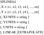
or
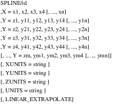
or
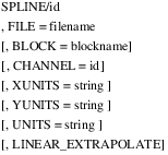
Arguments
BLOCK | Specifies the use of a particular, named block within a file. The BLOCK argument is optional, and requires the FILE argument. |
CHANNEL | For use with Adams Durability only. Specifies the integer ID of a particular channel of data in the file referenced by the SPLINE. This argument is used for files of type RPC III, which can contain more than one channel of data. An error results if the specified file is of type RPC and no CHANNEL argument is given or if the supplied channel ID does not exist in the file. Adams Solver ignores this argument for files of type DAC, which by definition contain only one channel of data. Default: (none) Range: 1 < n < 128 |
FILE | Specifies the use of a file, rather than the X and Y arguments, to supply data for the SPLINE. FILE causes Adams Solver (FORTRAN) to call the user-written subroutine SPLINE_READ, which you must provide. The FILE argument and the X and Y arguments are mutually exclusive. If you are using FILE with Adams Durability, it specifies the name of the time history file that supplies data for the the SPLINE. The file can be of type DAC (nSoft format) or RPC III (MTS format). For more on how to define a SPLINE using the FILE argument, see the example in SPLINE_READ subroutine. |
LINEAR_EXTRAPOLATE | Causes Adams Solver (FORTRAN) to extrapolate a SPLINE that exceeds a defined range by applying linear function(s) tangent to the spline at the end(s) of the defined range. By default, Adams Solver (FORTRAN) extrapolates a SPLINE that exceeds a defined range by applying a parabolic function over the first or last three data points. |
X=x1,x2,x3,x4[ , . . . , xn] | Specifies at least four x values. The maximum number of x values, n, depends on whether you specify a single curve or a family of curves. Values must be constants; Adams Solver (FORTRAN) does not allow expressions. Values must be in increasing order: x1 < x2 < x3, and so on. |
Y=y1,y2,y3,y4 [ , . . . , yn] | Approximates a single curve by specifying the corresponding y value: y1,y2,y3,y4[, . . . ,yn] for each x value. Values must be constants; Adams Solver (FORTRAN) does not allow expressions. |
Y=z1,y11,y12,y13,y14 [ , . . . , y1n] ,Y=z2,y21,y22,y23,y24 [ , . . . , y2n] ,Y=z3,y31,y32,y33,y34 [ ,ym1,ym2,ym3,ym4 [ , . . . , ymn]] | Approximates a family of curves by specifying the corresponding y values: y1,y2,y3,y4[, . . . ,yn] for the x values at unique z values (z1[, . . . ,zm]). Values must be constants; Adams Solver (FORTRAN) does not allow expressions. Values for z must be in increasing order: z1 < z2 < z3, and so on. |
UNITS | For use with Adams Durability only. Specifies the type of units to be used for all the sets of values. Valid values are: "angle", "force", "frequency", "length", "mass", "time", "inertia", "velocity", "acceleration", "angular_velocity", "angular_acceleration", "stiffness", "damping", "torsion_stiffness", "torsion_damping", "area", "volume", "torque", "pressure", "area_inertia", "density", "energy", "force_time", "torque_time", "flowrate_pressure_d", "flow_rate", "force_per_angle", "damping_per_angle". Default: (none) |
XUNITS YUNITS ZUNITS | Specify the type of units to be used for individual set of values (X, Y or Z respectively). In general X units will be “time” and Y units will be of type “length”. Valid values are: "angle", "force", "frequency", "length", "mass", "time", "inertia", "velocity", "acceleration", "angular_velocity", "angular_acceleration", "stiffness", "damping", "torsion_stiffness", "torsion_damping", "area", "volume", "torque", "pressure", "area_inertia", "density", "energy", "force_time", "torque_time", "flowrate_pressure_d", "flow_rate", "force_per_angle", "damping_per_angle". Default: (none) |
Extended Definition
Adams Solver (FORTRAN) applies curve-fitting techniques that interpolate between data points to create a continuous function. If the SPLINE data has one independent variable, Adams Solver (FORTRAN) uses a cubic polynomial to interpolate between points. If the SPLINE data has two independent variables, Adams Solver (FORTRAN) uses a cubic method to interpolate between points of the first independent variable, and then uses a linear method to interpolate between curves of the second independent variable.
The next sections explain more about using the SPLINE statement:
Using the Spline Function
To use discrete data input with a SPLINE statement, you must write either a function expression that includes one of the two Adams Solver (FORTRAN) spline functions (AKISPL and CUBSPL) or a user-written subroutine that calls one of the two spline data-access subroutines (AKISPL and CUBSPL).
Spline Function Interpolation Methods
The SPLINE functions and data-access subroutines use two different interpolation methods: the Akima method and a traditional cubic interpolation method.
■The AKISPL function and the AKISPL subroutine use the Akima method of interpolation. This method includes a local, cubic, curve-fitting technique.
■The CUBSPL function and the CUBSPL subroutine use the traditional cubic method of interpolation. This method includes a global, cubic, curve-fitting technique.
Both the Akima method and the traditional cubic method use cubic polynomials to interpolate values that fall between two adjacent points on a curve. Both provide closer approximations than other curve fitting techniques (for example, Lagrange polynomials, difference tables, and Fourier series). For data with two independent variables, Adams Solver (FORTRAN) uses linear interpolation to determine values that fall between curves.For more information about these curve-fitting techniques, see AKISPL and CUBSPL functions.
Using Spline with Adams Durability
The Adams Durability SPLINE statement is an extension of the Adams Solver (FORTRAN) SPLINE statement that supports the input of experimental test data from industry standard formats DAC and RPC III. The DAC format comes from nCode/nSoft. The RPC III file format comes from MTS.
DAC or RPC III files do not have standard file extensions. To determine which of these file types is in use, Adams Solver (FORTRAN) opens the file and reads a minimal amount of information contained in the file head. If the specified file is not of type DAC or RPC III, Adams Solver (FORTRAN) assumes that the file is a user-defined file format, and processes the SPLINE statement using a SPLINE_READ user-supplied subroutine. For more on how to define a SPLINE using the FILE argument for user-defined file formats, see the example in SPLINE_READ subroutine.
To use DAC or RPC III data that is specified in a SPLINE statement as input to Adams Solver (FORTRAN), you must write a function expression that includes the INTERP function. For more on how to use the Adams Durability INTERP function, see the INTERP function.
Tip: | When selecting points to represent a curve or a surface: ■Crowd points in regions with high rates of change. ■Spread out points in regions with slow rates of change. |
Caution: | The x and z data must cover the anticipated range of values. However, the following situations sometimes cause Adams Solver (FORTRAN) to evaluate a spline outside of its defined range: ■Adams Solver (FORTRAN) occasionally approximates partial derivatives using a finite differencing algorithm. ■Adams Solver (FORTRAN) occasionally attempts an iteration that moves the independent variable outside of its defined range. If this occurs, Adams Solver (FORTRAN) issues a warning message and extrapolates the four closest spline points. If the extrapolation is poor, Adams Solver (FORTRAN) may have difficulty reaching convergence, which may affect the results. To avoid these problems, try to use real points, and extend spline values 10 percent beyond the total dynamic range. |
Examples
The set of values in the table below relates the force in a spring to its deformation.
Data Relating Spring and Spring-Deflection Force
Deflection | Force |
-0.33 | -38.5 |
-0.17 | -27.1 |
-0.09 | -15.0 |
0.0 | 0.0 |
0.10 | 10.0 |
025 | 30.0 |
0.40 | 43.5 |
0.70 | 67.4 |
From this table, you can determine force when deflection equals -0.33, and you can determine force when deflection equals -0.17. However, what is the force when deflection equals -0.25?
To determine the force at any deflection value, Adams Solver (FORTRAN) creates a continuous function that relates deflection and force. This continuous approximation can evaluate the value of the spring force at a deflection of -0.25. If you input two sets of values (X and Y) with the SPLINE statement, then Adams Solver can effectively define the function as a curve. The following example illustrates how the SPLINE statement is used to store the discrete data in the table above.
SPLINE/01,
, X=-0.33, -0.17, -0.09, 0.0, 0.1, 0.25, 0.4, 0.7
, Y=-38.5, -27.1, -15.0, 0.0, 10.0, 30.0, 43.5, 67.4
, X=-0.33, -0.17, -0.09, 0.0, 0.1, 0.25, 0.4, 0.7
, Y=-38.5, -27.1, -15.0, 0.0, 10.0, 30.0, 43.5, 67.4
, XUNITS = “length”
, YUNITS = “force”
This SPLINE statement passes the data in the table above to a subroutine or function that uses cubic spline functions to fit a curve to the values. The curve allows Adams Solver (FORTRAN) to interpolate a value of Y for any value of X. It also specifies that the X values are of type length and Y values are of type force.
The set of values in the table below details a set of nonlinear, force-deflection relationships of a spring at various temperatures.
Data Relating Spring Force to Spring Deflections at Various Temperatures
Force at degrees Fahrenheit: | ||||
Deflection: | 20° | 30° | 40° | 50° |
-0.33 | -38.5 | -36.0 | -30.0 | -25.1 |
-0.17 | -27.1 | -25.4 | -21.7 | -18.6 |
-0.09 | -15.0 | -13.1 | -9.6 | -4.4 |
0.0 | 0.0 | 0.0 | 0.0 | 0.0 |
0.1 | 10.0 | 9.1 | 7.5 | 4.6 |
0.25 | 30.0 | 26.4 | 21.3 | 17.8 |
0.40 | 43.5 | 37.9 | 34.1 | 27.1 |
0.70 | 67.4 | 60.3 | 53.2 | 46.3 |
From table above, you can determine force when deflection equals -0.33 and when temperature equals 20°. You can also determine force when deflection equals -0.17 and when temperature equals 30°. However, what is the force when deflection equals -0.25 and when temperature equals 25°?
To determine the force at any deflection and temperature, you need to define a set of continuous functions that generally relate force to deflection and temperature. If deflection is the independent x value and temperature is the independent z value, you can define a set of functions in a family of curves using the SPLINE statement. The SPLINE statement for this example is shown next:
SPLINE/02,
, X=-0.33, -0.17, -0.09, 0.0, 0.10, 0.25, 0.40, 0.70
, Y=20, -38.5, -27.1, -15.0, 0.0, 10.0, 30.0, 43.5, 67.
, Y=30, -36.0, -25.4, -13.1, 0.0, 9.1, 26.4, 37.9, 60.3
, Y=40, -30.0, -21.7, -9.6, 0.0, 7.5, 21.3, 34.1, 53.2
, Y=50, -25.1, -18.6, -4.4, 0.0, 4.6, 17.8, 27.1, 46.3
, X=-0.33, -0.17, -0.09, 0.0, 0.10, 0.25, 0.40, 0.70
, Y=20, -38.5, -27.1, -15.0, 0.0, 10.0, 30.0, 43.5, 67.
, Y=30, -36.0, -25.4, -13.1, 0.0, 9.1, 26.4, 37.9, 60.3
, Y=40, -30.0, -21.7, -9.6, 0.0, 7.5, 21.3, 34.1, 53.2
, Y=50, -25.1, -18.6, -4.4, 0.0, 4.6, 17.8, 27.1, 46.3
This SPLINE statement passes the data in the table above to a subroutine or function that uses cubic spline functions to fit a curve to the y values at each set of x and z values.
Examples Using the SPLINE Statement with Adams Durability
The following examples require a licence for the Adams Durability plugin to Adams Solver (FORTRAN).
SPLINE/101,
FILE=test.dac
MOTION/6, I=401, J=402, B3
,FUNCTION=INTERP(TIME,3, 101)*DTOR
FILE=test.dac
MOTION/6, I=401, J=402, B3
,FUNCTION=INTERP(TIME,3, 101)*DTOR
The SPLINE statement defines a spline using test data supplied from a DAC file named test.dac. The MOTION statement controls the rotation of Marker 401 with respect to Marker 402 about the z-axis of Marker 401 using a function expression.
The function expression for the MOTION statement references data from the SPLINE statement using the INTERP function. The test data from the DAC file is known to be acquired in degrees, and since Adams Solver (FORTRAN) expects rotational motion to be specified in radians, a conversion from degrees to radians (factor DTOR) is also included in the function expression.
SPLINE/201,FILE=test.rpc,CHANNEL=1
SPLINE/202,FILE=test.rpc,CHANNEL=2
SPLINE/203,FILE=test.rpc,CHANNEL=3
MOTION/1, I=401, J=402, X, FUNCTION=INTERP(TIME,3,201)
MOTION/2, I=401, J=402, Y, FUNCTION=INTERP(TIME,3,202)
MOTION/3, I=401, J=402, Z, FUNCTION=INTERP(TIME,3,203)
SPLINE/202,FILE=test.rpc,CHANNEL=2
SPLINE/203,FILE=test.rpc,CHANNEL=3
MOTION/1, I=401, J=402, X, FUNCTION=INTERP(TIME,3,201)
MOTION/2, I=401, J=402, Y, FUNCTION=INTERP(TIME,3,202)
MOTION/3, I=401, J=402, Z, FUNCTION=INTERP(TIME,3,203)
This example defines three splines that reference three different channels of test data from the same RPC III file. Each of these splines supplies the test data to a MOTION statement using the INTERP function.
See other Reference data available.