GSE
The GSE (General State Equation) statement lets you represent a subsystem that has arrays of input variables (u), internal continuous states (xc), internal discrete states (xd), and output variables (y).
The GSE is represented mathematically in one of two ways. The first is described by Equations (1), (2), and (3) below. It is for systems in which the time derivative of the continuous states can be written explicitly, and it is thus known as an explicit GSE:
 | (1) |
 | (2) |
 | (3) |
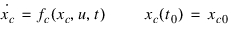
This is the default form. This is also the only form available for Adams Solver (C++) versions prior to Adams Solver version 2005r2 (and for any version of Adams Solver (FORTRAN)). The states xc are defined in Equation (1) as explicit, first-order, ordinary differential equations. The function fc(xc, u, t) is specified in a user-written subroutine, and is assumed to be continuous everywhere. (The names of this and other user-written subroutines are specified by the user via the ROUTINE or INTERFACE attributes of the GSE statement.) Integrators in Adams Solver (C++) evaluate fc(xc, u, t) as needed.
The states xd are defined in Equation (2) by the function fd(xd(n), u, tn). This function is specified in a second user-written subroutine. Equation (2) is a difference equation. A sampling period is associated with Equation (2), and integrators only evaluate Equation (2) at the sample times. The states xd are assumed to be constant between sampling periods. In Equation (2), xd(n) is the short form for xd(tn).
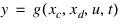
The outputs y are defined in Equation (3) by g(xc, xd, u, t), and are sampled continuously. This function is specified in a third user-written subroutine. It may be discontinuous in nature. If the outputs are to be fed back into the mechanical system through a force element, then it is customary to eliminate the discontinuities in y by passing the appropriate output variables through a low-pass filter before feeding those signals into the force element. You can use the TFSISO element to define a low-pass filter. Failure to eliminate discontinuities in y is likely to cause significant numerical-integration difficulties.
The second way (mentioned above) of representing a GSE mathematically is described by replacing Equation (1) above with (4) below:
 | (4) |
This representation permits the modeling of implicitly-defined states – a more general capability than what is possible with the default representation of Equation (1). This representation is thus known as an implicit GSE, and its use requires the inclusion of the IMPLICIT attribute of the GSE statement. Equations (2) and (3) are the same for explicit and implicit GSEs.
Note that the use (that is, interface) of the implicit form is more restricted than in the default case. Specifically, you must call the Array query utility subroutines: GSE_X, GSE_XDOT, GSE_XD, GSE_U() to obtain the values of 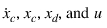 respectively, because the SYSARY subroutine does not support access to this data. As well, the Partial derivative entry utility subroutines: GSEPAR_X, GSEPAR_XDOT, GSEPAR_U must be called to supply the integrator with the partials of
  with respect to
  , respectively.
respectively, because the SYSARY subroutine does not support access to this data. As well, the Partial derivative entry utility subroutines: GSEPAR_X, GSEPAR_XDOT, GSEPAR_U must be called to supply the integrator with the partials of with respect to , respectively. If Equation (1) or (4) is not present, the GSE is classified as a purely discrete GSE. If Equation (2) is not present, the GSE is classified as being purely continuous. If both Equations 1(or 4) and 2 are present, the GSE is classified as a sampled system. When neither Equations 1( or 4) nor 2 are present, the GSE does not contain any internal states.
Format
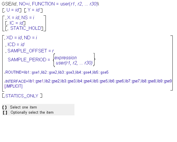
Arguments
FUNCTION=USER(r1[,...,r30]) | Specifies the parameters that are to be passed to the user-written subroutines that define the constitutive equations of a GSE. Two user subroutines are associated with a GSE. ■GSE_OUTPUT is called to evaluate g() in Equation (3). |
IC=id | Identifies the ARRAY statement in the dataset that specifies the initial conditions for the states in the system. This is an optional argument. When you use the IC argument, an ARRAY statement with this identifier must be in the dataset, it must be of the IC type, and it must have the number of elements specified in the argument NS. When you do not specify an IC array for a GSE statement, all the states are initialized to zero. |
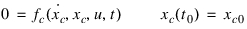
IMPLICIT | Specifies that the constitutive equation governing the states is implicitly defined and takes the form given in Equation (4). Note that the use of this attribute mandates that the GSE_XDOT and GSEPAR_XDOT utility subroutines get called by the user to obtain and supply required information. |
INTERFACE= lib1::gse_deriv, lib2::gse_output, lib3::gse_update, lib4::gse_samp, lib5::gse_set_ns, lib6::gse_set_nd, lib7::gse_set_implicit, lib8::gse_set_static_hold, lib9::gse_set_sample_offset | Specifies an alternative library and subroutine names for the user subroutines GSE_DERIV, GSE_OUTPUT, GSE_UPDATE, GSE_SAMP, GSE_SET_NS, GSE_SET_ND, GSE_SET_IMPLICIT, GSE_SET_STATIC_HOLD, GSE_SET_SAMPLE_OFFSET respectively. The rules for the INTERFACE argument are the same as for the ROUTINE argument. Learn more about the ROUTINE Argument. |
ND=i | Specifies the number of discrete states in the GSE. Discrete states are updated by calling the function GSE_UPDATE at the sample times. ND defaults to zero when not specified. |
NO=i | A mandatory argument, NO, specifies the number of output equations (algebraic variables) that are used in the definition of Equation 2. If NO is greater than 0, you must also specify a Y array. GSE outputs are evaluated by calling the user written subroutine GSE_OUTPUT. |
NS=i | |
ROUTINE=lib1::gse1, lib2::gse2, lib3::gse3, lib4::gse4, lib5::gse5 | Specifies alternative library and subroutine names for the deprecated user subroutines GSESUB, GSEXX, GSEXU, GSEYX, GSEYU respectively. Learn more about the ROUTINE Argument. |
SAMPLE_OFFSET=r | Specifies the simulation time at which the sampling of the discrete states is to start. All discrete states before SAMPLE_OFFSET are defined to be at the initial condition specified. SAMPLE_OFFSET defaults to zero when not specified. |
SAMPLE_PERIOD=expression | Specifies the sampling period associated with the discrete states of a GSE. This tells Adams Solver (C++) to control its step size so that the discrete states of the GSE are updated at: last_sample_time + sample_period In cases where an expression for SAMPLE_PERIOD is difficult to write, you can specify it in a user-written subroutine GSE_SAMP(…). Adams Solver (C++) will call this function at each sample time to find out the next sample period. |
STATIC_HOLD | Indicates that the continuous GSE states are not permitted to change during static and quasi-static simulations. |
U=id | Designates the ARRAY statement in the dataset that is used to define the input variables for the GSE. The U argument is optional. When it is not present in the GSE statement, there are no system inputs. When you use the U argument an ARRAY with this identifier must be in the dataset. The number of inputs to the GSE statement is inferred from the number of VARIABLE statements in the U array. |
X=id | Designates the ARRAY statement in the dataset that is used to define the states for the GSE. When you specify it, an ARRAY statement with this identifier must be in the dataset, it must be of the X type, and it may not be used in any other LSE, GSE, or TFSISO statement. If you specify SIZE on the ARRAY statement, it must have the same value as the argument NS. |
Y=id | Designates the ARRAY statement in the dataset that is used to define the output variables for the GSE. The Y argument is optional, but it must be provided if the argument NO is greater than zero. When it is not present in the GSE statement (and NO=0), there are no system outputs. When you use the Y argument, an ARRAY with this identifier must be in the dataset. If you specify SIZE on the ARRAY statement, it must have the same value as the argument NO. |
XD=id | Designates the ARRAY statement in the dataset that is used to access the discrete states for the GSE. An ARRAY statement with this identifier must be in the dataset, it must be of the X type, and it may not be used in any other LSE, GSE, or TFSISO statement. If you specify SIZE on the ARRAY statement, it must have the same value as the argument ND. |
STATICS_ONLY | When included (or set to On) will only activate GSE for statics. During dynamics the GSE will be inactive if set, and this should speed up the Solver solution during dynamics since less number of states are being solved. |
Extended Definition
The GSE (General State Equation) statement defines the equations for modeling a nonlinear, time varying, dynamic system. The statement is especially useful for importing nonlinear control laws developed manually or with an independent software package. It can also be used to define an arbitrary system of coupled differential and algebraic equations:
The GSE allows you to implement four different kinds of systems. These are:
Continuous Systems
Continuous systems can be represented either explicitly or implicitly. The explicit case is written in state-space form as:
 | (5) |
 | (6) |
where xc is called the state of the system, and contains n elements for an nth-order system. In matrix notation, xc is a column matrix of dimension n x 1. u defines the inputs to the system. Its size is equal to the number of inputs to the system being modeled. In this description, the system is assumed to have m inputs, consequently u is a column matrix of size m x 1. y defines the outputs from the system. If a system has p outputs, y is represented with a column matrix of dimension p x 1.
Using this system description, a nonlinear, second-order differential equation, with a single input u, such as:
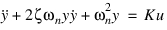 | (7) |
can be written in a state-space form as:
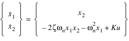 | (8) |
 | (9) |
The system state Equation (8) is integrated by Adams Solver using its integrators. Therefore, it is necessary that the functional relationship expressed in Equation (8) be continuous. This necessity is a minimum requirement for successfully integrating these equations. Similarly, if the output is to be fed back into a plant model, such as a mechanical system, Equation (9) is also required to be continuous. A higher degree of differentiability will help the integrators solve these equations more efficiently.
When the IMPLICIT attribute is present, the governing equations take the form of:
 | (10) |
 | (11) |
where all of the variables are defined equivalently to the explicit case above. The continuity requirements apply as well. For the implicit case, Equations (8) would be rewritten as:
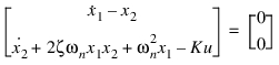 | (12) |
The major advantage of the implicit representation is that a more general set of equations can be solved because the dependence on the  terms can be nonlinear. A second advantage is that derivation of the state equations for a dynamical system in implicit rather than explicit form is usually easier, and the required partial derivatives of the state equations are usually much simpler expressions.
terms can be nonlinear. A second advantage is that derivation of the state equations for a dynamical system in implicit rather than explicit form is usually easier, and the required partial derivatives of the state equations are usually much simpler expressions.Discrete Systems
Discrete systems can be described by their difference equations. They are, therefore, represented in state-space form as:
 | (13) |
 | (14) |
xd is called the state of the system, and contains n elements for an nth-order system. In matrix notation, xd is a column matrix of dimension n x 1. u and y have the same meaning as for continuous systems.
The fundamental difference between continuous and discrete systems is that the discrete or digital system operates on samples of the sensed plant data, rather than on the continuous signal. The dynamics of the controller are represented by recursive algebraic equations, known as difference equations, that have the form of Equation (13).
The sampling of any signal occurs repetitively at instants in time that are  seconds apart.
  is called the sampling period of the controller. In complex systems, the sampling period is not a constant, but is, instead, a function of time and the instantaneous state of the controller. The signal being sampled is usually maintained at the sampled value in between sampling instances. This is called zero-order-hold. Determining an appropriate sampling period is a crucial design decision for discrete and sampled systems.
seconds apart. is called the sampling period of the controller. In complex systems, the sampling period is not a constant, but is, instead, a function of time and the instantaneous state of the controller. The signal being sampled is usually maintained at the sampled value in between sampling instances. This is called zero-order-hold. Determining an appropriate sampling period is a crucial design decision for discrete and sampled systems.One major problem to avoid with sampling is aliasing. This is a phenomenon where a signal at a frequency  produces a component at a different frequency
  only because the sampling occurs too infrequently. The general rule of thumb for such situations is as follows:
produces a component at a different frequency only because the sampling occurs too infrequently. The general rule of thumb for such situations is as follows:If you want to avoid aliasing in a signal with a maximum frequency of  , the sampling frequency
  is calculated from
  . This is an extreme lower limit for
  . If you want to obtain a reasonably smooth time response, then choose
  such that
  .
.
, the sampling frequency is calculated from . This is an extreme lower limit for . If you want to obtain a reasonably smooth time response, then choose such that .The sampling rate for sampling the states of a discrete system must follow the above criterion to avoid aliasing.
Note that when an Adams Solver output time and a GSE sample time coincide, the output of the GSE at that time will be calculated using the values of the discrete states before the update takes place. This is true for discrete states in discrete systems and sampled systems.
Sampled Systems
There are many systems that are neither continuous nor discrete. Some signals are sampled at discrete intervals, while others are sampled continuously. These systems are called sampled systems and are represented in state-space form as:
 | (15) |
 | (16) |
 | (17) |
 | (18) |
Equation (15) or (16) represents the dynamics associated with the continuous portion of the sampled system.
Equation (17) represents the dynamics associated with the discrete portion of the sampled system. The equations are evaluated only at discrete points in time: the sample times for the sampled system. In between sample times, the discrete states are assumed to be constant.
Equation (18) defines the outputs of the system. It is important to note that the Adams integrators evaluate Equation (18) as often as necessary. In many problems, it is required to examine the output between sampling instants. Often, for example, the maximum overshoot may occur not at a sampling instant, but between sampling instants. This implementation allows for such observations to be made on the output.
Feed-Forward Only System
Feed-Forward Only Systems are systems that have no internal states. The output of the system is an algebraic function of the inputs. They can be represented as:
 | (19) |
Integrator step size selection
When discrete GSE elements are included in a model, the integrators (GSTIFF, HHT and so on.) will select the next time step taking into account the sample period of each GSE in the model. The process is as follows, first the integrator will compute and propose a time step using its standard approach. Next the proposed time step will be compared with all of the sample periods proposed by the GSE elements in the model. Finally, the integrator will compute the step size making sure the system will not step beyond the sample period of any GSE. In a case of the constant sample period, the sample period of each discrete GSE in the model should be chosen such that the output step size (DTOUT) is an integer multiple of the sample period for optimal solver performance. In a case of multiple discrete GSEs with constant sample periods, the sample periods should be selected as the integer multiples of each other. Please note that these recommendations are made for optimal solver performance only. The integrators will honor any sample period set by the user.
Caution: | ■The GSE statement provides a very general capability for modeling nonlinear systems. However, the routines for solving the linear equations in Adams Solver (C++) have been developed and refined to work particularly well with the sparse systems of equations that come from the assembly of mechanical models. With the GSE statement, you can create very dense sets of equations. If these equations form a large portion of the completed model, Adams Solver (C++) may perform more slowly than expected. ■To improve the performance of Adams Solver (C++), any arrays of partial derivatives which are not full can be represented in sparse form. This sparse form can substantially reduce the effort required by the integrator. To represent the partials in sparse form, use the GSEMAP_* utility subroutines, when calling GSE_DERIV with IFLAG=1, to define the sparsity. Then, use the GSEPAR_* utility subroutines to pass the sparse partial arrays to the integrator. ■During a static analysis, Adams Solver (C++) finds equilibrium values for user-defined differential variables (DIFFs, GSEs, LSEs, and TFSISOs), as well as for the displacement and force variables. This changes the initial conditions for a subsequent analysis. If STATIC_HOLD is not specified, during a static analysis, Adams Solver (C++) sets the time derivatives of the user-defined variables to zero, and uses the user-supplied initial-condition values only as an initial guess for the static solution. Generally, the final equilibrium values are not the same as the initial condition values. Adams Solver (C++) then uses the equilibrium values of the user-defined variables as the initial values for any subsequent analysis, just as with the equilibrium displacement and force values. However, the user-specified initial conditions are retained as the static equilibrium values when STATIC_HOLD is specified. Thus, the final equilibrium values are the same as the user-specified initial conditions. Note that this does not guarantee that the time derivatives of the user-defined variable are zero after static analysis. |
Examples
Modeling Control Systems
The example below demonstrates how you can use a GSE to define a controller in Adams. The plant consists of a block on a translational joint. A control force is to be applied to the block so that it translates exactly 150 mm from its initial position. The control system is defined as follows.
Inputs
■The first input (u1) is the location of the block.
■The second input (u2) is the velocity of the block.
Outputs
■The output is an actuator signal.
States
■The controller is a linear PID controller.
■It has two continuous states (x1 and x2).
Transfer Functions
The transfer functions for the controller is:
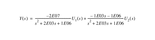
Putting the above equation in state-space representation, we obtain:
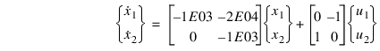
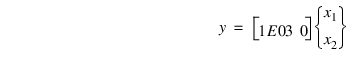
Or


In this example, a GSE will be used to define the state-space representation of the controller. Using DATA statements, matrices [A], [B] are entered in the GSE’s function GSE_DERIV, while matrix [C] is entered in the GSE’s function GSE_OUTPUT (see code below). Standard Adams modeling elements PART, JOINT, and SFORCE represent the block, translational joint, and the actuator, respectively.
Model Input File
GSE Test: Continuous states=2, Discrete states=0, Outputs=1
units/force=newton, mass=kilogram, length=millimeter, time = second
part/1, ground
marker/3, part = 1, reuler = 90d, 90d, 0d
marker/5, part = 1, qp = -150, 0, 0, reuler = 90d, 90d, 0d
part/2, qg = 0, 0, -100, mass = 46, cm = 6, ip = 2e5, 5e5, 4e5
marker/2, part = 2, qp = 0, 0, 100, reuler = 90d, 90d, 0d
marker/4, part = 2, qp = -150, 0, 100, reuler = 90d, 90d, 0d
marker/6, part = 2, qp = 0, 0, 100
marker/7, part = 2, qp = -150, 0, 100
joint/1, trans, i = 2, j = 3
sforce/1, trans, i = 4, j = 5, actiononly, function = aryval(2,1)
variable/2, function = dx(7)
variable/3, function = vx(7)
array/1, u, size = 2, variables = 2, 3 !Inputs for the GSE
array/2, y, size = 1 !Outputs for the GSE
array/3, x, size = 2 !States for the GSE
gse/99, ns = 2, no = 1, x = 3, u = 1, y = 2, function = user(3,1)
accgrav/jgrav = -9806.65
results/formatted
END
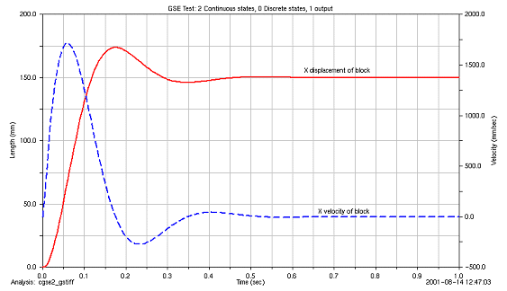
The figure below shows the time history of the location and velocity of the block. Notice the displacement (red curve) starts at 0 mm, and stops moving when it reaches a value of 150 mm. Notice also the overshoot in the displacement of the block, which is subsequently corrected by the controller.
Time History of the Block Location
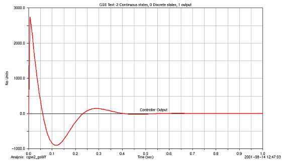
The next figure shows the time history of the actuator signal computed by the controller. This is the force applied on the block. Notice that the actuator signal changes sign when the block is about to overshoot its target value.
Time History of Actuator Signal Output by the Controller
User-Written Subroutines for the controller modeled by GSE
SUBROUTINE GSE_DERIV(ID, TIME, PAR, NPAR, DFLAG, IFLAG, NS, XDOT)
C
C Inputs:
C
INTEGER ID, NPAR, NS
DOUBLE PRECISION PAR(*), TIME
LOGICAL IFLAG, DFLAG
C
C Outputs:
C DOUBLE PRECISION XDOT(*)
C
C Local Variables:
C
LOGICAL LEFLAG, PARFLG
INTEGER AX(1), AU(1), NSS, NU
DOUBLE PRECISION A(2,2), B(2,2), X(2), U(2)
SAVE A, B
DATA A /-1.0e3, 0.0, -2.0e4, -1.0e3/
DATA B /0.0, 1.0, -1.0, 0.0/
C
C+-----------------------------------------------------------------*
C
C Define the function fc():
C
AX(1) = NINT(PAR(1))
AU(1) = NINT(PAR(2))
CALL SYSARY ('ARRAY', AX, 1, X, NSS, LEFLAG)
CALL SYSARY ('ARRAY', AU, 1, U, NU, LEFLAG)
XDOT(1) = A(1,1)*X(1)+A(1,2)*X(2) + B(1,1)*U(1)+B(1,2)*U(2)
XDOT(2) = A(2,1)*X(1)+A(2,2)*X(2) + B(2,1)*U(1)+B(2,2)*U(2)
C
C Return the partial derivatives to ADAMS:
C
CALL ADAMS_NEEDS_PARTIALS (PARFLG)
IF (PARFLG) THEN
CALL SYSPAR ('ARRAY', AX, 1, A, NSS*NSS, LEFLAG)
CALL SYSPAR ('ARRAY', AU, 1, B, NSS*NU , LEFLAG)
ENDIF
RETURN
END
C
C+================================================================*
C
SUBROUTINE GSE_OUTPUT (ID, TIME, PAR, NPAR, DFLAG, IFLAG, NO, Y)
C
C Inputs:
C
INTEGER ID, NPAR, NO
DOUBLE PRECISION PAR(*), TIME
LOGICAL IFLAG, DFLAG
C
C Outputs:
C
DOUBLE PRECISION Y(NO)
C
C Local Variables:
C
LOGICAL LEFLAG, PARFLG
INTEGER AX(1), NS
DOUBLE PRECISION C(2), X(2)
SAVE C
DATA C/1.0e3, 0.0/
C
C+--------------------------------------------------------------*
C
C Define the function g():
C
AX(1) = NINT(PAR(1))
CALL SYSARY ('ARRAY', AX, 1, X, NS, LEFLAG)
Y(1) = C(1)*X(1) + C(2)*X(2)
C
C Return the partial derivatives to ADAMS:
C
CALL ADAMS_NEEDS_PARTIALS (PARFLG)
IF (PARFLG) THEN
CALL SYSPAR ('ARRAY', AX, 1, C, NS, LEFLAG)
ENDIF
C
C
RETURN
END
Modeling Control Systems - Implicit formulation
This example models the same system in the example immediately above with an implicit formulation. This is an extremely simple model, but it serves to highlight the differences. In general, the A, B, and E matrices need not be constant, and the E matrix need not be diagonal.
In the .adm file, all that needs to be changed is the addition of the IMPLICIT attribute to the GSE statement.
gse/99, IMPLICIT, ns = 2, no = 1, x = 3, u = 1, y = 2, function = user(3,1)
For the implicit case, the GSE_DERIV user-supplied subroutine needs to be changed as follows (note comments included in the code):
SUBROUTINE GSE_DERIV(ID, TIME, PAR, NPAR, DFLAG, IFLAG, NS, F)
C
C Inputs:
C
INTEGER ID, NPAR, NS
DOUBLE PRECISION PAR(*), TIME
LOGICAL IFLAG, DFLAG
C
C Outputs:
C
DOUBLE PRECISION F(*)
C
C Local Variables:
C
LOGICAL LEFLAG, PARFLG
INTEGER NStates, NInputs, i, j
DOUBLE PRECISION A(2,2), B(2,2), X(2), U(2), E(2,2), XDOT(2)
SAVE A, B
DATA A /-1.0e3, 0.0, -2.0e4, -1.0e3/
DATA B /0.0, 1.0, -1.0, 0.0/
DATA E /-1.0D0, 0.0D0, 0.0D0, -1.0D0/
C
C+--------------------------------------------------------------------*
C
C Explicit form of governing equation: Xdot = A*X + B*U
C Implicit form is: 0 = A*x + B*U + E*Xdot
C
C
C Query the utility subroutines for the number of states and inputs.
C
CALL GSE_NS (NStates)
CALL GSE_NI (NInputs)
C
C Query the utility subroutines for the current values of the state, time derivative of state and input vectors.
C
CALL GSE_X (X, NStates)
CALL GSE_XDOT (Xdot, NStates)
CALL GSE_U (U, NInputs)
C
C Construct the return vector, f, in implicit form
C
DO i=1, NStates
F(i) = 0.0D0
DO j = 1, NStates
F(i) = F(i) + A(i,j)*X(j) + B(i,j)*U(j) + E(i,j)*Xdot(j)
ENDDO
ENDDO
C
C Return the partial derivatives to ADAMS:
C
CALL ADAMS_NEEDS_PARTIALS (PARFLG)
IF (PARFLG) THEN
CALL GSEPAR_X (A, NStates*NStates)
CALL GSEPAR_XDOT (E, NStates*NStates)
CALL GSEPAR_U (B, NStates*NInputs)
ENDIF
RETURN
END
Of course, the results of the implicit and explicit formulations are identical to within roundoff error.
Modeling Control Systems – Implicit formulation with sparse representation of partial arrays
As a final example, this case again models the same system, again implicitly, but this time uses the GSEMAP_* utility subroutines to specify the sparse representation of the partial derivative arrays.
Notes: | 1. There is no attribute or other keyword used to specify a sparse representation. The use of a GSE_MAP_* utility subroutine implies a sparse representation for that array. 2. Sparse and non-sparse representations can be mixed. As in this example, the E matrix can be represented sparsely while the others are represented as full. |
The only change to the previous example is in the GSE_DERIV user-supplied subroutine. In this case it looks like:
SUBROUTINE GSE_DERIV(ID, TIME, PAR, NPAR, DFLAG, IFLAG, NS, F)
C
C Inputs:
C
INTEGER ID, NPAR, NS
DOUBLE PRECISION PAR(*), TIME
LOGICAL IFLAG, DFLAG
C
C Outputs:
C
DOUBLE PRECISION F(*)
C
C Local Variables:
C
LOGICAL LEFLAG, PARFLG
INTEGER NStates, NInputs, i, j
DOUBLE PRECISION A(2,2), B(2,2), X(2), U(2), E(2), XDOT(2)
SAVE A, B
DATA A /-1.0e3, 0.0, -2.0e4, -1.0e3/
DATA B /0.0, 1.0, -1.0, 0.0/
DATA E /-1.0D0, -1.0D0/
C
C+--------------------------------------------------------------------*
C
C Explicit form of governing equation: Xdot = A*X + B*U
C Implicit form is: 0 = A*x + B*U + E*Xdot
C
C
C Specify a sparse representation for the E matrix
C
IF (IFLAG) then
CALL GSEMAP_XDOT(1,1)
CALL GSEMAP_XDOT(2,2)
ENDIF
C
C Query the utility subroutines for the number of states and inputs.
C
CALL GSE_NS (NStates)
CALL GSE_NI (NInputs)
C
C Query the utility subroutines for the current values of the state, time derivative of state and input vectors.
C
CALL GSE_X (X, NStates)
CALL GSE_XDOT (Xdot, NStates)
CALL GSE_U (U, NInputs)
C
C Construct the return vector, f, in implicit form
C
DO i=1, NStates
F(i) = 0.0D0
DO j = 1, NStates
F(i) = F(i) + A(i,j)*X(j) + B(i,j)*U(j)
ENDDO
F(i) = F(i) + E(i)*Xdot(i)
ENDDO
C
C Return the partial derivatives to ADAMS:
C
CALL ADAMS_NEEDS_PARTIALS (PARFLG)
IF (PARFLG) THEN
CALL GSEPAR_X (A, NStates*NStates)
CALL GSEPAR_XDOT (E, NStates )
CALL GSEPAR_U (B, NStates*NInputs)
ENDIF
RETURN
END
Again, the results are identical to the previous two examples to within roundoff error.
See other Generic systems modeling available.