Using the 521-Tire Model
About 521-Tire
The 521-Tire model is a simple model that requires a small set of parameters or experimental data to simulate the behavior of tires. The 521-Tire is the first tire model incorporated in Adams. The name “521” (actually “5.2.1”) refers to the version number of Adams Tire when it was first released.
The slip forces and moments can be calculated in two ways:
■Using the Equation method
■Using the Interpolation method
Two dedicated contact methods exist for the 521-Tire:
■Point Follower, used for Handling analysis models
■Equivalent Plane Method, used for 3D Contact analysis models
Any combination of force and contact method is allowed.
The road data files used for the 521-Tire are unique and cannot be used in combination with any other Handling tire model. The 521 road file format is described in Road Data File 521_pnt_follow.rdf.
Note that the capability and generality of the 521-Tire have been superseded by other, newer tire models, described throughout this guide. We’ve retained the 521-Tire model primarily for backward compatibility. We recommend that you use other tire models for new work.
Definition of Tire Slip Quantities
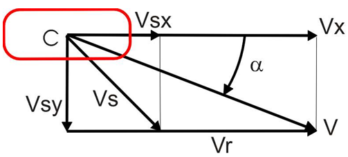
Figure 1 Slip Quantities at Combined Cornering and Braking/Traction
The longitudinal slip velocity Vsx in the SAE-axis system is defined using the longitudinal speed Vx, the wheel rotational velocity  , and the loaded rolling radius Rl:
, and the loaded rolling radius Rl: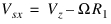 | (1) |
The lateral slip velocity is equal to the lateral speed in the contact point with respect to the road plane:
 | (2) |
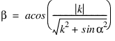
The practical slip quantities  (longitudinal slip) and
  (slip angle) are calculated with these slip velocities in the contact point:
(longitudinal slip) and (slip angle) are calculated with these slip velocities in the contact point: 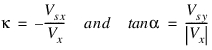 | (3) |
Note that for realistic tire forces the slip angle  is limited to 90 degrees and the longitudinal slip
  in between -1 (locked wheel) and 1.
is limited to 90 degrees and the longitudinal slip in between -1 (locked wheel) and 1.Force Calculations
You can use the 521-Tire model for handling and durability analyses.
Directional Vectors for the Application of Tire Forces and Torques at the Center of the Tire-Road Surface Contact Patch
Figure 2 Tire Forces and Torques at the Center of the Tire-Road Surface Contact Patch
The forces act along the directional vectors. From the tire spin vector and various information you supply in the tire property and the road profile data files, Adams Tire determines the positions and orientations of the tire vertical, lateral, and longitudinal directional vectors. Figure 2 shows these directional vectors.
The tire vertical force acts along the vertical directional vector, the tire aligning torque acts about the same vector, the tire lateral force acts along the lateral directional vector, and the tire longitudinal force acts along the longitudinal directional vector. At this point, Adams Tire determines the force directions as if it were going to apply the tire aligning torque and all of the tire forces at the center of the tire-road surface contact patch.
The tire-road surface contact patch may deflect laterally. Adams Tire calculates the lateral deflection in the direction (and with the sign) of the lateral force. The magnitude of the deflection is equal to the lateral force divided by the tire lateral stiffness you provide in the tire property data file.
The tire vertical, lateral, and longitudinal forces are forces in the tire vertical, lateral, and longitudinal directions (as determined at the tire-road surface contact patch). The tire aligning torque is a torque about the tire vertical vector. The vehicle durability force has components in both the tire vertical and the tire longitudinal directions.
Normal Force
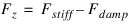
The tire normal force Fz is calculated based on the tire deflection and radial velocity. A progressive spring and linear damping constant are employed:
 | (4) |
where Fstiff is tire stiffness force and Fdamp is tire damping force. The vertical stiffness force is calculated from:
 | (5) |
where Kz is the tire vertical stiffness, δ is tire deflection, and  is the stiffness exponent. The tire damping force is calculated from:
is the stiffness exponent. The tire damping force is calculated from: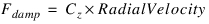 | (6) |
where Cz is the tire damping constant.
The damping constant is reduced for small tire deflections, which are below 5% of the unloaded tire radius.
The tire vertical stiffness can also be described using a spline function (force versus deflection) in the Adams dataset. The user array is used to switch between tire property file stiffness and spline stiffness. If the first value in the user array is equal to '5215', the spline vertical stiffness is used. The second value of the user array refers to the ID of the spline. The message, 'Using spline data for the vertical spring', is shown in the message file. If the first value in the user array is not equal to '5215', the tire property file stiffness is used.
The following is an example of using the spline vertical stiffness:
! adams_view_name='spline_vertical_stiffness'
SPLINE/10
, X = -1,0,10,30
, Y = 0,0,2000,6000
!
! adams_view_name='wheel_user_array'
ARRAY/102
, NUM=5215,10
Another option for having a non-linear tire stiffness is to introduce a deflection-load table in the tire property file in a section called [DEFLECTION_LOAD_CURVE]. See 521-Tire Tire and Road Property Files. If a section called [DEFLECTION_LOAD_CURVE] exists, the load deflection datapoints with a cubic spline for inter- and extrapolation are used for the calculation of the vertical force of the tire.
Longitudinal Force
The tire longitudinal force Fx can have up to three contributions:
■Traction/braking force
■Rolling resistance force
■Durability force (in case of durability contact)
Traction/Braking Force
Traction force is developed if the vehicle is starting to move and a braking force if the vehicle is beginning to stop. In either case, the absolute magnitude of the force is calculated from:
 | (7) |
where the friction coefficient μ is a function of the longitudinal slip velocity Vsx in the contact patch. Note that this is somewhat unusual, since all the other Handling tire models in Adams Tire assume that the longitudinal force Fx is a function of the slip ratio.
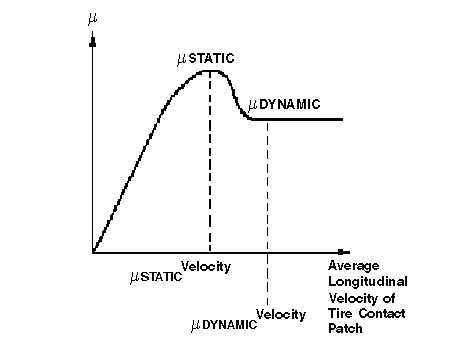
Figure 3 Schematic of Friction Coefficient Versus Local Slip Velocity
The μ curve as a function of longitudinal slip velocity is created using standard Adams STEP functions (see body 4 on page 10). You have to specify two points on the curve to define this characteristic:
■The coordinates of the curve at μstatic: (velocity μstatic, μstatic)
■The coordinates of the curve at μdynamic: (velocity μdynamic, μdynamic)
The friction values may be available to you as function of slip ratio instead of slip velocity. Converting Slip Ratio Data to Velocity Data explains how the slip ratios can be converted to slip velocities.
Rolling Resistance Force
Rolling resistance Moment My is calculated from:
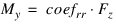 | (8) |
where coefrr is the rolling resistance coefficient that should be supplied in the tire property data file.
Durability Force
Durability force, sometimes known as radial planar force, is a special kind of tire vertical force. It is the durability force that resists the action of road bumps. This force acts along the instantaneous vertical directional vector calculated by Adams Tire. The Adams Tire durability tire forces are limited to two-dimensional forces that lie in the plane of the tire and are directed toward the wheel-center marker. Adams Tire superimposes these forces upon any traction or lateral forces developed in the tire-road surface interaction.
You must select the Equivalent Plane Method for generating these durability forces.
Lateral Force and Aligning Torque
Two methods exist for calculating the lateral force Fy and self-aligning moment Mz:
■Interpolation Method
■Equation Method
Interpolation Method
The AKIMA spline is employed to calculate Fy and Mz as a function of the slip angle α, camber angle γ, and vertical load Fz. You should provide the data in the SAE axis system.
Note that the slip angle α and vertical load Fz input for the force and moment calculation of Fx, Fy, Mx, My, and Mz are limited to minimum and maximum values in the input to avoid unrealistic extrapolated values.
Equation Method
The Equation Method uses the following equation to generate the lateral force Fy:
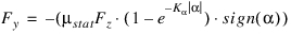 | (9) |
where Kα denotes the tire cornering stiffness coefficient.
The aligning moment Mz is calculated using the pneumatic trail t according to:
 | (10) |
while the pneumatic trails are calculated with half the contact length a:
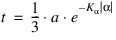 | (11) |
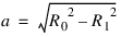 | (12) |
with R0 and Rl are, respectively, the unloaded and loaded tire radius.
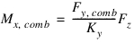
Overturning Moment
In both methods, the overturning moment Mx calculation is based on the lateral tire force Fy, the lateral tire stiffness Ky, and the vertical load:
 | (13) |
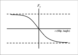
Figure 4 Tire Lateral Force as a Function of Slip Angle
■The contribution of the camber  is disregarded in the Equation Method.
is disregarded in the Equation Method.■The cornering stiffness equals  .
.
.Combined Slip of 5.2.1
The combined slip calculation of the 5.2.1. is using the friction ellipse and is similar to the combined slip calculation of the Pacejka '89 and '94 tire models.
Inputs:
■Dimensionless longitudinal slip  (range -1 to 1) and side slip angle
  in radian
(range -1 to 1) and side slip angle in radian ■Longitudinal force Fx and lateral force Fy calculated using the equations of 521-Tire
■The vertical shift of Fy,α=0 is Fy calculated at zero slip angle
Output:
■Adjusted longitudinal force Fx and lateral force Fy incorporates the reduction due to combined slip:
■
Friction coefficients:
 | (14) |
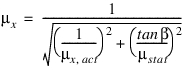 | (15) |
Forces corrected for combined slip conditions:
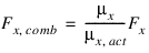 | (16) |
Due to the lateral deflection of the tire patch, the aligning moment under combined slip conditions increases by the effect of the longitudinal force Fx and the lateral tire stiffness Ky:
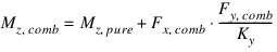 | (17) |
and the overturning moment uses the lateral force for combined slip:
 | (18) |
Transient Behavior in the 5.2.1 Tire Model
In the upper sections described force calculations are valid for the 'so-called' steady-state tire response, in other words tire dynamics is not taken into account. However, in general, the tire will be exposed to changes of input in terms of vertical load and longitudinal and lateral slip continuously.
For estimating transient tire behavior, a linear transient model is used as described in [1].
In the linear transient model the tire contact point S' is suspended to the wheel-rim plane with a longitudinal and lateral spring, with respectively stiffness's CFx and CFy. In the figure below a top view of the tire with the single contact point S' and the longitudinal (u) and lateral (v) carcass deflections is shown.
Figure 5 Transient Behavior in the 5.2.1 Tire Model
The contact point may move with respect to the wheel-rim plane and road. Movements relative to the road will result in tire-road interaction forces. Differences in slip velocities at point S and point S' will result in the tire carcass to deflect. The change of the longitudinal deflection u can be defined as:
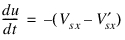 | (19) |
and the lateral deflection v as:
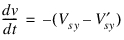 | (20) |
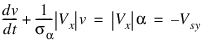
For small values of slip the side force Fy can be calculated using the cornering stiffness CFα as follows:
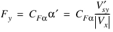 | (21) |
While the lateral force on the carcass reads:
 | (22) |
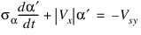
When introducing the lateral relaxation length σα as:
 | (23) |
the differential equation for the lateral deflection can be written as follows:
 | (24) |
For linear small slip we can define the practical slip quantity α' as:
 | (25) |
With α' the equation for the lateral deflection becomes:
 | (26) |
Similar the differential equation for longitudinal direction with the longitudinal relaxation length σκ can be derived:
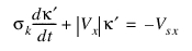 | (27) |
with the practical slip quantity 
 | (28) |
These practical slip quantities  and
and  are used instead of the usual
  and
and  definitions for steady-state tire behavior.
and are used instead of the usual and definitions for steady-state tire behavior. The longitudinal and lateral relaxation length are read from the tire property file, see Tire Property File 521_equation.tir and 521_interpol.tir.
Note that in transient mode the tire model is able to deal with zero speed (stand-still), because this linear transient model works with tire deflections instead of slip velocities.
The effective lateral compliance of the tire at stand-still in transient mode is:
 | (29) |
And similar in longitudinal direction the compliance is:
 | (30) |
Smoothing
When you indicate smoothing by setting the value of USE_MODE in the tire property file, Adams Tire smooths initial transients in the tire force over the first 0.1 seconds of the simulation. The longitudinal force, lateral force, and aligning torque are multiplied by a cubic step function of time. (See STEP in the Adams Solver online help.)
■Longitudinal Force Fx = SFx
■Lateral Force Fy = SFy
■Overturning moment torque Mx = SMz
■Aligning torque Mz = SMz
Changing the Operating Mode: USE_MODE
You can change the behavior of the tire model by changing the value of USE_MODE in the [MODEL] section of the tire property file. If USE_MODE equals zero, or when it is absent, the smoothing time equals 0.001 seconds and the 521-Tire model is compatible with the previous Adams Solver implementation.
By selecting a value of USE_MODE between 1 and 4, smoothing and combined slip correction can be switched on and off, as shown in Table 1. The smoothing time equals 0.1 seconds for these values of USE-MODE.
If the USE_MODE is larger then 10, the tire model will account for the relaxation length effects (transient tire response).
USE_MODE | Smoothing | Combined slip correction | Tire response |
|---|---|---|---|
1 | off | off | Steady-state |
2 | off | on | Steady-state |
3 | on | off | Steady-state |
4 | on | on | Steady-state |
11 | off | off | Transient |
12 | off | on | Transient |
13 | on | off | Transient |
14 | on | on | Transient |
Converting Slip Ratio Data to Velocity Data
Adams Tire requires that you enter the velocities that correspond to μstatic and μdynamic. You will often obtain this information as the coefficient of friction versus slip ratio. You can calculate the velocities required by Adams Tire from the coefficient of friction versus slip ratio curve in the following way:
 | (31) |
where
■ = Slip ratio
= Slip ratio■ = Free rolling rotational velocity (no slip)
= Free rolling rotational velocity (no slip)■ = Actual rotational velocity
= Actual rotational velocityKinematic relationships between translational and rotational velocities and the effective rolling radius give:
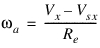 | (32) |
 | (33) |
where
■ = Contact patch velocity reletive to road surface
= Contact patch velocity reletive to road surface■ = Actual longitudinal velocity
= Actual longitudinal velocity■ = Effective rolling radius
= Effective rolling radiusSubstituting these relationships into the original slip ratio equation with some cancelling of variables gives:
 | (34) |
Therefore:
 | (35) |
During testing for the coefficient of friction as a function of slip ratio, the longitudinal velocity Vx is held constant. Therefore, you can obtain Vsx, the relative velocity of the contact patch with respect to the road surface, from the test data curves for the static and dynamic values of friction.
Contact Methods
For handling analyses (which use a flat road surface profile), the 521-Tire model uses the point-follower contact method. For durability analyses (which use uneven road surface profiles), the Equivalent Plane Method yields the instantaneous tire radius directly, while finding the new road surface orientation vector.
About the Point-Follower Method
The point-follower contact method assumes a single contact point between the tire and road. The contact point is the point nearest to the wheel center that lies on the line formed by the intersection of the tire (wheel) plane with the local road plane.
The contact force computed by the point-follower contact method is normal to the road plane. Therefore, in a simulation of a tire hitting a pothole, the point-follower contact method does not generate the expected longitudinal force.
About the Equivalent Plane Method
521-Tire uses the Equivalent Plane method to reorient the vertical road surface vector, which gives the direction of the vertical force, and to calculate the new tire radius. To do this, a new smooth road surface is generated at an angle calculated such that only the shape of the tire is different (see body 6 on page 18).
Figure 6 Equivalent Plane Method
Both the deflected tire area and its centroid remain unchanged. The vector between the deflected area centroid and the wheel-center marker then determines the orientation of the. vertical vector perpendicular to the road surface.
The Equivalent Plane method is best suited for relatively large obstacles because it assumes the tire encompasses the obstacle uniformly. In reality, the pneumatics and the bending stiffness of the tire carcass prevent this. The result is an uneven pressure distribution and possibly gaps between the tire and the road. If the obstacle is larger than the tire contact patch (such as a pothole or curb), the uniform assumption is good. If the obstacle is much smaller than the tire patch, however (such as a tar strip or expansion joint), the assumption is poor, and the Equivalent Plane method may greatly underestimate the durability force.
Definition of Equivalent Plane Parameters
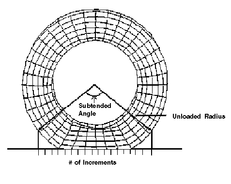
Figure 7 Equivalent Plane Parameters
When using the Equivalent Plane method the following parameters need to be specified in the tire property file:
Equivalent_plane_angle
Specifies the subtended angle (in degree) bisected by the z-axis of the wheel-center marker, as shown in Figure 7. This angle determines the extent of the road the tire can envelop. The value of the equivalent_plane_angle must be between 0 and 180 degrees.
Equivalent_plane_increments
Specifies the number of increments into which the shadow of the tire subtended section is divided, as shown in Figure 7.
521-Tire Tire and Road Property Files
This section contains four example input data files. For reference, the files are called:
■521_equation.tir
■521_interpol.tir
■521_pnt_follow.rdf
■521_equiv_plane.rdf
The first two files are tire property files, and the last two are road files. The file 521_equation.tir illustrates the required format and parameters when you use the Equation method. The file 521_interpol.tir illustrates the Interpolation method. The two *.rdf files show how road data files must be specified when either of the contact methods is used.
Tire Property File 521_equation.tir and 521_interpol.tir
You can select the method for calculating the normal force by setting the VERTICAL_FORCE_METHOD parameter to either POINT_FOLLOWER (for the Point Follower method) or EQUIVALENT_PLANE (for the Equivalent Plane method). See Contact Methods for details on these methods.
You can select the method for calculating the lateral force by setting the LATERAL_FORCE_METHOD parameter to either INTERPOLATION or symbol. See Lateral Force and Aligning Torque for details on these calculation methods.
The following table specifies how some of the parameter names used in the tire property file correspond to parameters introduced in the equations that were presented in the previous sections.
Parameter in file: | Used in equation: | As parameter: |
|---|---|---|
vertical_stiffness | Kz | |
vertical_damping | Cz | |
lateral_stiffness | Ky | |
cornering_stiffness_coefficient | Kα | |
Mu_Static | μstatic | |
Mu_Dynamic | μdynamic | |
Mu_Static_velocity | velocity μstatic | |
Mu_Dynamic_Velocity | velocity μdynamic | |
rolling_resistance_coefficient | coeffrr | |
unloaded_radius | R0 | |
relax_length_x |  | |
relax_length_y |  | |
vertical_stiffness_exponent |  Note: If you do not specify vertical_stiffness_exponent in the tire property file, 521-Tire uses the default value of 1.1. |
521-equation.tir
The 521-equation.tir example tire property file starts here.
$----------------------------------------------------------MDI_HEADER
[MDI_HEADER]
FILE_TYPE = 'tir'
FILE_VERSION = 3.0
FILE_FORMAT = 'ASCII'
(COMMENTS)
{comment_string}
'Tire - XXXXXX'
'Pressure - XXXXXX'
'Test Date - XXXXXX'
'Test tire'
$---------------------------------------------------------------units
[UNITS]
LENGTH = 'mm'
FORCE = 'newton'
ANGLE = 'rad'
MASS = 'kg'
TIME = 'second'
$---------------------------------------------------------------model
[MODEL]
! use mode 1 2 3 4 11 12 13 14
! ------------------------------------------------------------------
! smoothing X X X X
! combined X X X X
! transient X X X X
!
PROPERTY_FILE_FORMAT = '5.2.1'
USE_MODE = 1
$-----------------------------------------------------------dimension
[DIMENSION]
UNLOADED_RADIUS = 310.0
WIDTH = 195.0
ASPECT_RATIO = 0.70
RIM_RADIUS = 195,0
RIM_WIDTH = 139.7
$----------------------------------------------------------parameters
!
VERTICAL_FORCE_METHOD = EQUIVALENT_PLANE
LATERAL_FORCE_METHOD = EQUATION
!
vertical_stiffness = 206.0
vertical_stiffness_exponent = 1.1
vertical_damping = 2.06
!
lateral_stiffness = 50
cornering_stiffness_coefficient = 50
!
Mu_Static = 0.95
Mu_Dynamic = 0.75
Mu_Static_Velocity = 3000
Mu_Dynamic_Velocity = 6000
!
rolling_resistance_coefficient = 0.01
!
EQUIVALENT_PLANE_ANGLE= 100
EQUIVALENT_PLANE_INCREMENTS= 50
!
RELAX_LENGTH_X = 500.0
RELAX_LENGTH_Y = 300.0
521_interpol.tir
The 521-interpol.tir example tire property file starts here. In addition to the file for 521_equation.tir, it contains data that is used for calculating the lateral force and aligning moment, instead of using formula 6 to 9. Note that the [DEFLECTION_LOAD_CURVE] can also be used in the tire property file for the Equation method.
$----------------------------------------------------------MDI_HEADER
[MDI_HEADER]
FILE_TYPE = 'tir'
FILE_VERSION = 3.0
FILE_FORMAT = 'ASCII'
(COMMENTS)
{comment_string}
'Tire - XXXXXX'
'Pressure - XXXXXX'
'Test Date - XXXXXX'
'Test tire'
$---------------------------------------------------------------units
[UNITS]
LENGTH = 'mm'
FORCE = 'newton'
ANGLE = 'rad'
MASS = 'kg'
TIME = 'second'
$---------------------------------------------------------------model
[MODEL]
! use mode 1 2 3 4 11 12 13 14
! ----------------------------------------------------------------
! smoothing X X X X
! combined X X X X
! transient X X X X
!
PROPERTY_FILE_FORMAT = '5.2.1'
USE_MODE = 1
$-----------------------------------------------------------dimension
[DIMENSION]
UNLOADED_RADIUS = 310.0
WIDTH = 195.0
ASPECT_RATIO = 0.70
RIM_RADIUS = 195,0
RIM_WIDTH = 139.7
$----------------------------------------------------------parameters
!
VERTICAL_FORCE_METHOD = POINT_FOLLOWER ! or EQUIVALENT_PLANE
LATERAL_FORCE_METHOD = INTERPOLATION ! or EQUATION
!
vertical_stiffness = 206.0
vertical_stiffness_exponent = 1.1
vertical_damping = 2.06
lateral_stiffness = 50
cornering_stiffness_coefficient = 50
!
Mu_Static = 0.95
Mu_Dynamic = 0.75
Mu_Static_Velocity = 3000
Mu_Dynamic_Velocity = 6000
!
rolling_resistance_coefficient = 0.01
!
EQUIVALENT_PLANE_ANGLE= 100
EQUIVALENT_PLANE_INCREMENTS= 50
!
RELAX_LENGTH_X = 500.0
RELAX_LENGTH_Y = 300.0
!
!------------------CAMBER ANGLE VALUES-------------------------------
! Conversion
! No. of pnts factor(D to R) pnt1 pnt2 pnt3 pnt4 pnt5
!
CAMBER_ANGLE_DATA_LIST
5 0.017453292 -3.0 0.0 3.0 6.0 10.0
!
!------------------SLIP ANGLE VALUES---------------------------------
! Conversion
! No. of pnts factor(D to R) pnt1 ...... pnt9
!
SLIP_ANGLE_DATA_LIST
9 0.017453292 -15.0 -10.0 -5.0
-2.5 0.0 2.5
5.0 10.0 15.0
!
!-----------------VERTICAL FORCE VALUES------------------------------
! Conversion
! No. of pnts factor
! pnt1 pnt2 pnt3 pnt4 pnt5
!
VERTICAL_FORCE_DATA_LIST
5 4.448
200.0 600.0 1100.0 1500.0 1900.0
!
!-----------------ALLIGNING TORQUE VALUES---------------------------
! No. of pnts Conversion
! factor
!
! pnt1 .... pnt225
!
ALIGNING_TORQUE_DATA_LIST
225 -1355.7504
5.31 6.52 22.88 26.41 30.58
0.11 2.84 5.49 -3.92 -14.04
0.47 -12.44 -37.99 -67.22 -116.07
0.04 -21.38 -69.04 -111.44 -168.11
0.80 -3.70 -27.94 -44.25 -53.74
1.75 17.43 52.20 81.97 145.78
2.54 11.08 40.53 73.54 95.55
-1.28 0.02 14.82 2.93 10.35
1.59 -3.77 -17.17 6.60 -11.91
0.06 14.23 22.93 11.45 15.74
5.95 5.54 13.72 -1.65 -15.64
-1.29 -9.45 -26.98 -57.25 -107.71
-5.05 -17.73 -62.62 -109.03 -161.88
0.46 -2.48 -19.48 -33.54 -49.52
4.71 26.10 60.80 90.85 119.51
4.26 16.60 52.46 93.32 141.34
2.41 4.28 2.21 9.11 30.44
-0.92 0.22 12.61 2.51 -18.77
0.43 -4.62 15.36 7.16 11.70
6.70 15.92 0.14 -4.20 -11.81
-2.20 -5.53 -13.28 -47.48 -92.88
-1.39 -17.28 -52.17 -102.80 -161.71
2.87 -0.38 -14.27 -29.03 -42.42
6.99 24.54 66.06 93.27 126.38
7.10 18.78 58.20 104.51 156.39
1.63 2.91 8.33 20.32 42.09
-0.78 10.13 -9.94 -13.02 -11.95
5.62 4.36 23.16 38.03 8.73
2.31 6.41 14.10 6.03 -11.66
7.87 1.33 -16.31 -40.24 -82.58
1.40 -10.04 -50.94 -93.06 -157.50
2.10 0.56 -16.15 -27.15 -40.13
5.60 26.48 62.92 90.16 122.03
3.56 20.63 60.74 108.26 162.97
-0.08 1.81 14.39 34.98 59.72
1.38 -2.13 -2.42 -4.08 -2.72
3.69 1.71 29.06 10.05 11.38
3.09 7.15 -7.92 13.53 -5.78
6.08 0.38 -2.69 -32.10 -62.17
0.76 -7.65 -37.28 -89.05 -145.09
0.70 4.37 -7.59 -23.71 -28.49
5.92 34.39 72.55 92.88 129.34
4.36 29.81 76.70 118.91 180.59
-2.03 5.94 26.18 53.59 89.76
0.39 -5.52 -6.06 10.16 7.81
!-----------------LATERAL FORCE VALUES------------------------------
! No. of pnt Conversion
! factor
! pnt1 .... pnt225
!
LATERAL_FORCE_DATA_LIST
225 4.448
234.08 585.56 1000.29 1307.77 1603.78
269.79 628.82 1040.78 1331.72 1624.83
213.70 565.29 974.49 1198.82 1387.74
150.79 452.18 752.21 885.23 960.13
11.52 50.58 199.87 199.50 208.75
-116.75 -367.42 -618.68 -683.16 -857.81
-224.15 -588.24 -1001.01 -1235.88 -1488.88
-242.08 -612.70 -1059.55 -1344.53 -1658.66
-213.99 -597.29 -988.14 -1343.86 -1689.35
234.40 572.75 981.30 1352.37 1698.90
239.27 647.77 1007.37 1357.22 1666.30
252.34 603.75 1033.50 1288.76 1483.64
167.55 481.45 826.41 962.64 1028.74
32.23 78.77 231.31 250.14 254.32
-122.59 -423.13 -552.58 -613.52 -607.61
-208.93 -576.28 -948.45 -1149.44 -1314.69
-261.05 -634.90 -1064.15 -1338.52 -1581.84
-241.50 -607.16 -1021.87 -1322.30 -1598.25
210.20 578.56 968.72 1344.05 1730.40
237.91 600.60 1025.67 1377.57 1733.03
226.60 629.48 1084.97 1354.12 1575.22
154.74 496.21 878.72 1028.03 1095.59
34.37 74.19 240.00 284.42 283.85
-130.29 -339.00 -509.04 -543.75 -555.05
-226.48 -557.52 -884.91 -1083.18 -1175.12
-270.70 -595.22 -1059.76 -1314.74 -1564.43
-254.64 -602.76 -1032.71 -1313.22 -1609.96
238.28 531.25 945.70 1305.28 1786.96
227.13 594.51 1038.87 1365.33 1733.29
221.76 633.49 1135.31 1375.28 1619.82
195.50 505.90 899.88 1059.92 1135.28
28.51 68.59 241.99 311.15 331.84
-145.10 -319.56 -464.11 -499.27 -500.83
-230.33 -548.99 -815.88 -991.78 -1108.36
-230.62 -597.10 -1009.76 -1261.43 -1504.09
-218.36 -570.13 -1049.72 -1344.94 -1589.60
228.49 564.69 954.06 1332.84 1687.50
221.19 595.52 1019.74 1378.35 1749.40
224.63 590.58 1108.01 1408.87 1707.09
178.96 474.70 918.87 1125.97 1242.75
42.58 65.26 230.69 306.58 428.45
-144.43 -290.91 -368.02 -398.98 -394.66
-224.99 -494.65 -761.78 -886.03 -941.20
-246.51 -563.13 -980.33 -1249.57 -1462.88
-239.34 -567.10 -1050.56 -1348.66 -1611.11
521-Tire Road Data Files
The road data files used with the 521-Tire are unique and cannot be used with any other tire model. The data files are fully described by the following two examples.
Road Data File 521_pnt_follow.rdf
This example file shows that, if you use the Point Follower method and indicate it in the associated tire property file, the road_profile_type parameter must be set to FLAT.
$--------------------------------------------------------MDI_HEADER
[MDI_HEADER]
FILE_TYPE = 'rdf'
FILE_VERSION = 5.00
FILE_FORMAT = 'ASCII'
(COMMENTS)
{comment_string}
'flat 2d contact road for testing purposes'
$-------------------------------------------------------------UNITS
[UNITS]
LENGTH = 'mm'
FORCE = 'newton'
ANGLE = 'radian'
MASS = 'kg'
TIME = 'sec'
$-------------------------------------------------------------MODEL
[MODEL]
METHOD = '5.2.1'
FUNCTION_NAME = 'ARC913'
$--------------------------------------------------------PARAMETERS
ROAD_PROFILE_TYPE = FLAT
INITIAL_HEIGHT = 0.000
Road Data File 521_equiv_plane.rdf
The following example shows which data the road data file must contain if the Equivalent Plane method is used and specified in the associated tire property file. The main difference with the road data file used in association with the Point Follower method is that here the ROAD_PROFILE_TYPE parameter is set to INPUT and a ROAD_INPUT_DATA_LIST is specified.
$---------------------------------------------------------MDI_HEADER
[MDI_HEADER]
FILE_TYPE = 'rdf'
FILE_VERSION = 5.00
FILE_FORMAT = 'ASCII'
(COMMENTS)
{comment_string}
'5.2.1 input road for testing purposes'
$--------------------------------------------------------------UNITS
[UNITS]
LENGTH = 'mm'
FORCE = 'newton'
ANGLE = 'radian'
MASS = 'kg'
TIME = 'sec'
$--------------------------------------------------------------MODEL
[MODEL]
METHOD = '5.2.1'
FUNCTION_NAME = 'ARC913'
$---------------------------------------------------------PARAMETERS
ROAD_PROFILE_TYPE = INPUT
INITIAL_HEIGHT = 0.000
ROAD_INPUT_DATA_LIST
23, 1
-10000.00, 00.00
1740.00, 00.00
1740.94, 1.92
1743.73, 3.55
1748.31, 4.59
1754.55, 4.79
1762.32, 3.88
1771.41, 1.65
1781.61, 7.89
1792.65, 2.47
1804.28, 5.26
1816.20, 6.20
1828.12, 5.26
1839.75, 2.47
1850.79, 7.89
1860.99, 1.65
1870.08, 3.88
1877.85, 4.79
1884.09, 4.59
1888.67, 3.55
1891.46, 1.92
1892.40, 00.00
40000.00, 00.00