Adams Basic Package > Adams View > Adams View > Testing Models > Simulation Basics > About Simulation Output

About Simulation Output

When you perform a Simulation of your model in Adams View, think of it as performing a physical test of your physical model. When you perform a physical test, you add instrumentation, such as gauges and meters, so you can measure and extract useful information. You also examine the data in detail through plots to see if your design performed as you expected it to.

The same is true in Adams View. Adams Solver is automatically set up to output generic information to help you evaluate the quality of your design. You can also customize the output to obtain more specific information. In general, you should set up the output for any information you think is useful for model verification or system analysis.

Learn about:

■Default Simulation Results

■About Customizing Simulation Output

■Comparison of Measures and Requests

■Results Set Components

Default Simulation Results

The Simulation results that Adams Solver generates by default include:

■Characteristics of objects in your model - Object characteristics return basic information about parts, forces, and constraints in your model. For example, they return information about the position of the center of mass of a part.

Note:

Object characteristics correspond directly to object measures. You do not need to create object measures to plot object characteristics because Adams Solver automatically calculates and outputs them for you. To use object measures in the definition of your model or to save the object characteristics from one simulation to another, however, you should create object measures. Learn about measuring object characteristics.

■Result set components - Result set components are a basic set of state variable data that Adams Solver calculates during a simulation. Adams Solver outputs the data at each simulation output step. A component of a result set is a time series of a particular quantity (for example, the x displacement of a part or the y torque in a joint). Learn about result set components.

About Customizing Output

You can do the following to customize the output from a Simulation:

■Define measures that Adams View tracks during and after a simulation. You can measure almost any characteristic of the objects in your model, such as the force applied by a spring or the distance or angle between objects. As you run the simulation, Adams View displays strip charts of the measures so you can view the results as the simulation occurs. Learn About Measures.

■Create requests to ask for standard displacement, velocity, acceleration, or force information that helps you investigate the results of your simulation. You can also define other quantities (such as pressure, work, energy, momentum, and more) that you want output during a simulation. (Learn more about Creating Requests.)

■Define FE model data to be output for use in third-party programs. Learn about Defining FE Model Data for Output.

Measures are more flexible than requests. Besides specifying output, you can use measures in the definition of your model. Requests, on the other hand, let you specify several types of output through one request. (See comparison of requests and measures.)

Note:

You can also use the Measure Distance command to measure the distance between two markers at different model configurations. This is a quick way to measure distances and does not require that you run a simulation. For more information, see About Measuring Distance Between Positions.

Comparison of Measures and Requests
Measures:	Requests:
Measure one component.	Measure up to six components.
Have a variety of different predefined types.	Have only four types: Displacement, Velocity, Acceleration, or Force.
Can be used when plotting and in the definition of your model.	Can only be used when plotting.
Can be viewed during and after a simulation.	Can only be viewed after a simulation.
Correspond to VARIABLE statements, VARVAL functions, and REQUEST statements in Adams Solver.	Correspond to REQUEST statements in Adams Solver.

Result Set Components
For:	Calculated information is:
Joints, motion generators, applied loads, and flexible connectors
■Translational components (force):	■FX - X component of force ■FY - Y component of force ■FZ - Z component of force ■FMAG - Magnitude of force
■Rotational components (torque):	■TX - X component of torque ■TY - Y component of torque ■TZ - Z component of torque ■TMAG - Magnitude of torque
Screw joint, rackpin joint, rotational motion, gear, coupler, torsional spring-damper, bushing, beam, and field	Additional angle outputs. These outputs are the total angular displacements of the element. They are more than +/-360 degrees if the object twists more than one turn.
	For the element:	Component name(s):
	Screw joint	ANG
	Rackpin joint	ANG
	Rotational motion	ANG
	Gear	ANG1, ANG2
	Coupler	ANG1, ANG2, ANG3
	Torsional spring-damper	ANG
	Bushing	ANGX, ANGY, ANGZ
	Beam	ANGX, ANGY, ANGZ
	Field	ANGX, ANGY, ANGZ
Parts
■Displacement	■X - X translational component ■Y - Y translational component ■Z - Z translational component ■MAG - Magnitude ■PSI - First rotation angle ■THETA - Second rotation angle ■PHI - Third rotation angle Note: PSI, THETA, and PHI are automatically associated with a body-fixed 313 rotation sequence. Uses measures or requests to obtain rotation angles associated with different rotation sequences.
■Velocity	■VX - X translational component ■VY - Y translational component ■VZ - Z translational component ■WX - X rotational component ■WY - Y rotational component ■WZ - Z rotational component
■Acceleration	■ACCX - X translational component ■ACCY - Y translational component ■ACCZ - Z translational component ■WDX - X rotational component ■WDY - Y rotational component ■WDZ - Z rotational component Note: All the results that Adams Solver calculates automatically for parts measure the movement of the part’s local coordinate system, not its center of mass. You should use measures or Requests if you want to measure the movement of a part’s center of mass.

Object Characteristics You Can Measure

In general, all objects in your model have some pre-defined measurable characteristics. For example, you can capture and investigate the power consumption of a motion, or measure a part’s center-of-mass velocity along the global x-axis, taking time derivatives in the ground reference frame. The default coordinate system is the ground coordinate system, but you can use any marker as the reference coordinate system.

The measurable characteristics of objects are shown in the table below. Click an object characteristic to view the description.

The object:	Has these measurable characteristics:
Rigid body	■CM_Position ■CM_Velocity ■CM_Acceleration ■CM_Angular_Velocity ■CM_Angular_Acceleration ■Kinetic_Energy ■Translational_Kinetic_ Energy ■Angular_Kinetic_Energy ■Translational_Momentum ■Angular_Momentum_ About_CM ■Potential_Energy_Delta
Point mass body	■CM_Position ■CM_Velocity ■CM_Acceleration ■Kinetic_Energy ■Translational_Kinetic_ Energy ■Translational_Momentum ■Potential_Energy_Delta
Flexible body	■CM_Position ■CM_Velocity ■CM_Acceleration ■CM_Angular_Velocity ■CM_Angular_Acceleration ■Kinetic_Energy ■Translational_Kinetic_ Energy ■Angular_Kinetic_Energy ■Translational_Momentum ■Angular_Momentum_ About_CM ■Potential_Energy_Delta ■Strain_Energy
Spring-damper force, single-component force, field force, bushing force	■element_force ■element_torque ■translational_displacement ■ax_ay_az_projection_ angles ■translational_velocity ■translational_acceleration ■Angular_Velocity ■Angular_Acceleration
Joint constraint, joint primitive constraint	■element_force ■element_torque ■translational_displacement ■translational_velocity ■translational_acceleration ■Angular_Velocity ■Angular_Acceleration ■ax_ay_az_projection_ angles
Curve-curve constraint, point-curve constraint	■pressure_angle ■element_force ■contact_point_location
Joint motion, general point motion	■power_consumption ■element_force ■element_torque ■translational_displacement ■translational_velocity ■translational_acceleration ■Angular_Velocity ■Angular_Acceleration ■ax_ay_az_projection_ angles
Three-component force, three-component torque, general force/torque	■element_force ■element_torque
Contact force	■element_force ■element_torque ■Double-click a track to view: ■I_Point ■I_Normal_Force ■I_Friction_Force ■I_Normal_Unit_Vector ■I_Friction_Unit_Vector ■J_Point ■J_Normal_Force ■J_Friction_Force ■J_Normal_Unit_Vector ■J_Friction_Unit_Vector ■Slip_Deformation ■Slip_Velocity ■Penetration

Point Characteristics You Can Measure

The object:	Has these measurable characteristics:
Marker	■Total_Force_On_Point ■Total_Force_At_Location ■Total_Torque_On_Point ■Total_Torque_At_Location ■Translational_Displacement ■Translational_Velocity ■Translational_Acceleration ■Angular_Velocity ■Angular_Acceleration

Object Measure Characteristic Descriptions

The following table describes the characteristics that object measures provide. For information on the conventions used, see Conventions.

Characteristics:	Description:	Definition/Formula:
CM_Position	Position vector of body's center of mass relative to the global origin.
CM_Velocity	Translational velocity vector of body's center of mass relative to the reference frame that you specify.
CM_Acceleration	Acceleration of body's center of mass relative to the reference frame that you specify.
CM_Angular_Velocity	Angular velocity of body's center-of-mass marker that you specify relative to the reference frame. Note: The center-of-mass marker is only important for flexible bodies. For rigid bodies, angular velocity is independent of the marker used.
CM_Angular_Acceleration	Angular acceleration of body's center of mass marker relative to the reference frame that you specify. Note: The center-of-mass marker is only important for flexible bodies. For rigid bodies, angular acceleration is independent of the marker used.
Kinetic_Energy	Total kinetic energy of body	(Translational _Kinetic_Energy + Angular_Kinetic_Energy) Note: For a flexible body, Adams View obtains the value directly from Adams Solver without performing additional calculations.
Translational_Kinetic_ Energy	Body's kinetic energy due to translational velocity only	Note: For a flexible body, this value is approximate because the translational and angular velocity cannot be separated from the general motion of the flexible body in the presence of deformation.
Angular_Kinetic_Energy	Body's kinetic energy due to angular velocity only	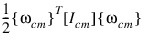Note: For a flexible body, this value is approximate because the translational and angular velocity cannot be separated from the general motion of the flexible body in the presence of deformation.
Translational_Momentum	Body's momentum due to translational velocity only
Angular_Momentum_ About_CM	Body's angular momentum due to angular velocity only	Note: For a flexible body, this value may be approximate, depending on how [Icm] is computed.
Potential_Energy_Delta	Body's current change in potential energy from time = 0
Strain_Energy	Flexible body's strain energy
CM_Position_Relative_ To_Body	Deformed position of flexible body's center of mass relative to undeformed position
element_force	Element force vector { FX , FY , FZ } relative to the reference frame that you specify
element_torque	Element torque vector { TX , TY , TZ } relative to the reference frame that you specify
translational_displacement	Translational displacement of Marker I with respect to Marker J, relative to the reference frame that you specify. Note: The displacement is with respect to the global origin.
ax_ay_az_projection_ angles	Rotational displacement (in model units) of Marker I about the x-axis, y-axis, or z-axis, respectively, of Marker J. Note: These angles are projections onto planes and are not associated with any rotation sequence (such as Body 3-1-3). You typically use them to measure planar moments.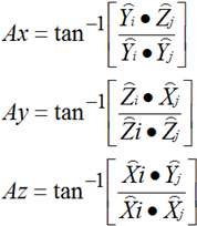
translational_velocity	Translational velocity vector of Marker I with respect to Marker J, in the reference frame that you specify
translational_acceleration	Translational acceleration vector of Marker I with respect to Marker J, in the reference frame that you specify
angular_velocity	Angular velocity vector of Marker I with respect to Marker J, in the reference frame that you specify
angular_acceleration	Angular acceleration vector of Marker I with respect to Marker J, in the reference frame that you specify
power_consumption	Total power consumed by motion.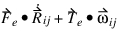
pressure_angle	Acute angle (in model units) between the line of motion of the follower and the normal to the cam surface at the point of contact between the cam and the follower (represented by angle α in the figure). Also, in the figure: ■Line MM is the line of motion of the follower. ■Line NN is the normal to line TT (the tangent).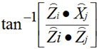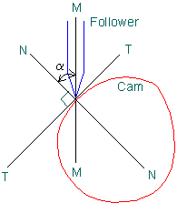
contact_point_location	Instantaneous point of contact (location of floating marker)	Currently not available
I_Point/J_Point	■I_Point defines the instantaneous contact point location on the body containing the I geometry for a given contact track. Components x, y, and z are provided. ■J_Point defines the instantaneous contact point on the body containing the J geometry for the same track. Components x, y, and z are provided. By default, all coordinates are calculated in the ground coordinate system. Furthermore, the common normal passes through both points.	Picture
I_Normal_Force/ J_Normal_Force	■I_Normal_Force defines the contact normal force acting at I_Point, in the direction of I_Normal_Unit_Vector (see below). Components x, y, z, and magnitude are provided. ■J_Normal_Force defines the contact normal force acting at J_Point. (It is equal but opposite to I_Normal_Force.) By default, all force components are calculated in the ground coordinate system.
I_Friction_Force/ J_Friction_Force	■I_Friction_Force defines the contact friction force acting at I_Point. The direction of the friction force is specified by I_Friction_Unit_Vector (see below). ■J_Friction_Force defines the contact friction force acting at J_Point. The direction of the friction force is specified by J_Friction_Unit_Vector (see below). (It is equal but opposite to I_Friction_Force.) Additional information provided: ■Mu - The instantaneous coefficient of friction at the contact point. ■Torque - The net friction torque caused by the friction forces acting about the contact point; it opposes the boring_velocity. By default, all force components are calculated in the ground coordinate system.
I_Normal_Unit_Vector/ J_Normal_Unit_Vector	■I_Normal_Unit_Vector defines the direction of the surface or curve normal at I_Point. This is also the direction of I_Normal_Force. ■J_Normal_Unit_Vector defines the direction of the surface or curve normal at J_Point. This is also the direction of J_Normal_Force. (It is opposite to the direction of I_Normal_Unit_Vector.) By default, all direction cosines (x, y, z) are calculated in the ground coordinate system.
I_Friction_Unit_Vector/ J_Friction_Unit_Vector	■I_Friction_Unit_Vector defines the direction of slip at I_Point. I_Friction_Force opposes motion of the body containing IGEOM in this direction. ■J_Friction_Unit_Vector defines the direction of slip at J_Point. J_Friction_Force opposes motion of the body containing JGEOM in this direction. By default, all direction cosines (x, y, z) are calculated in the ground coordinate system.
Slip_Deformation	Defines the three components and magnitude of the deformation vector at the contact point since the onset of stiction. Slip_Deformation is undefined during dynamic friction, and its components are set to zero.
Slip_Velocity	Defines the three components and speed (that is, magnitude) of the slip velocity vector at the contact point. By definition, this vector is orthogonal to the contact normal force.
Penetration	Defines kinematic information pertaining to the two geometries in contact. Three pieces of information are provided. ■Depth - The distance between the I_Contact Point and the J_Contact_Point. ■Velocity - The penetration velocity at the contact point. This is the relative velocity along the common normal at the contact point. ■Boring_Velocity - This is angular velocity about the common normal of the two geometries at the contact point.
Total_Force_On_Point	Returns the total force acting on a body via the marker referenced by the measure. If you have two forces acting on a body in the same location, and both forces use the same marker, then the total force at point will be the sum of the two forces. If a third force also acts at the same point but was created using a different marker, then this third force will not be considered in the first measure. For example, see Simcompanion Knowledge Base Article KB8016139.
Total_Force_At_Location	Returns the sum of all forces acting on a body at a specified location, regardless of how many markers are involved. For example, see Simcompanion Knowledge Base Article KB8016139.
Total_Torque_On_Point	This is the same as Total_Force_On_Point except the force is angular.
Total_Torque_At_Location	This is the same as Total_Force_At_Location except the force is angular.
Translational_Displacement	Position vector of marker relative to the global origin.
Translational_Velocity	Translational velocity vector of marker relative to the global reference frame.
Translational_Acceleration	Acceleration of marker relative to the global reference frame.
Angular_Velocity	Angular velocity of marker relative to the global reference frame. Note: The marker is only important for flexible bodies. For rigid bodies, angular velocity is independent of the marker used.
Angular_Acceleration	Angular acceleration of marker relative to the global reference frame. Note: The marker is only important for flexible bodies. For rigid bodies, angular acceleration is independent of the marker used.

Conventions for Measure Characteristics

The measure characteristics in Measure Characteristic Descriptions use the following conventions.

The characters:	Represent:
M	Total mass of a body.
cm	The center of mass of a body. Note: For flexible bodies, the location of the center of mass changes over time relative to the body coordinate system.
[Icm]	Inertia tensor of body about its center of mass. Note: For flexible bodies, the inertia tensor actually changes as the body deforms. Adams View accounts for this by correcting the inertia tensor of the flexible body, [I] according to its specified modal formulation as follows: ■Rigid or Constant: [I] = [I]7 ■Partial Coupling: [I] = [I]7 - [I]8 {q} ■Full Coupling: [I] = [I]7 - [I]8{q} - [I]9 {q}.{q}T The resulting [I] is then transformed from the local body reference frame (LBRF) to the body's center of mass (cm) to obtain [Icm].
	Change in position of the center of mass of the rigid body relative to its original position (at time=0).
{q}	Generalized modal coordinates of active modes of flexible body (modal deformations).
[K]	Generalized modal stiffness matrix of flexible body.
	Prescribed gravity vector.
	Unit vectors of marker I's x-, y-, and z-axis, respectively.
	Unit vectors of marker J's x-, y-, and z-axis, respectively.
N	Current number of time steps.
Mi	Measured data value in time step i.
Mn	Measured data value at the current time step n.
[I]2	Second invariant matrix of flexible body representing the undeformed center of mass scaled by the total mass.
[I]3	Third invariant matrix of flexible body representing the modal components of the flexible body's mass.
[I]7	Seventh invariant matrix of the flexible body representing the undeformed moment of inertia tensor in the LBRF.
[I]8	Eighth invariant matrix of the flexible body representing the first-order corrections to the inertia tensor due to modal deformation.
[I]9	Ninth invariant matrix of the flexible body representing the second-order corrections to the inertia tensor [I]7 due to modal deformation.

About Contact Result Tracks

A track is a sequence of individual impacts between two particular geometries specified by a single contact object. The two geometries for a particular track should always be the same at every impact along that track.

It is possible for a contact object and two of its geometries to have more than one track. For example, if a contact and two of its geometries have more than one impact at the same time, each separate impact must belong to a separate track to remove ambiguity. Also, when the separation between impacts is great enough according to either an automatic or given criteria, the impacts may be assembled into separate tracks.

There is an experimental method of specifying a delta value for the separation criteria that will make the program skip the automatic criteria, sometimes saving a significant amount of time. This can be done by setting the tolerance parameter using the analysis collate_contacts command. By using a large tolerance value, you can coerce tracks together that may have been separated by the automatic criteria. See Simcompanion Knowledge Base Article KB8015944 for more information.

Automatic criteria for a contact and an I and J geometry:

1. The geometric center (centroid) of all the impacts over the entire simulation is found in three frames: the global frame and the I and J part frames.

2. The average distance of the impacts from the centroid is computed, again in each of the three frames.

3. The standard deviation of the impacts from this average distance is computed in the three frames.

This value for the standard deviation is used as a delta to decide if any two impacts are close enough to be considered to belong to the same track. The frame with the minimum distance is used for the comparison.

To force a pair of locations on two different parts to belong to separate tracks you can place a small separate piece of geometry at that particular point on each part. For example, instead of making a table out of a single piece of geometry and letting the algorithm try to find the separate legs as four separate tracks, placing a cap at the end of each leg will force separate tracks.

Defining FE Model Data for Output

You can also set up Adams View to produce data files of component loads, deformations, stresses, or strains for input to subsequent finite-element or fatigue-life analysis for use in third-party products. You use the Settings -> Solver -> Output -> More -> Durability command to specify the type of file to produce. Adams View will not output to any files unless you specify the format.

To output FE model data:

1. From the Build menu, point to Data Elements, point to FEMdata, and then select either New or Modify.

The Create FEMDATA dialog box appears.

2. In the Name text box, enter the name of the FEMDATA element in the modeling database to create or modify.

3. Set Type to the information you want to output, and then enter the values in the dialog box as explained in the FEMDATA Output Dialog Box Options Table, depending on the type of format.

4. In the File text box, enter the output file name for the FEM data. You can specify an existing directory, root name, and/or extension. By default, the file name will be composed of the Adams run ID and body ID according to the type of data and file format that you specified in the Solver -> Settings -> Output -> More -> Durability Files.

5. Specify the start and end times for outputting the data:

♦From - Enter the time at which to start outputting the data. The default is the start of the simulation.

♦To - Enter the time at which to end the output of the data or the search of a peak load. The default is to output to the end of the simulation.

6. Select OK.