Example of Animating Natural Frequencies
The following example demonstrates how to view natural frequencies. In the example, you import an Adams View command file of a two-mass, two-degree of freedom (DOF) model. The model is shown in Figure 5.
In the model, a spring damper, SPRING_1, connects the larger part, PART_2, to the smaller part, PART_3. Another spring damper, SPRING_2, connects PART_3 to ground2. Both parts slide with respect to the ground in translational joints, JOINT_1 and JOINT_2, respectively.
In this example, you will load a command file that builds the model for you. You then use the Adams View linear modes controls to view the different modes in the model and plot and view a table of the eigenvalues.
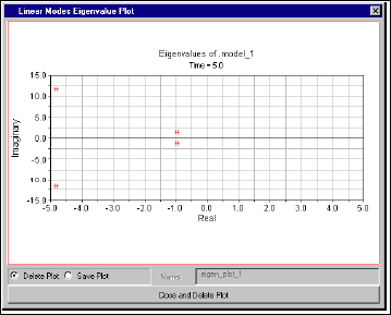
Figure 5 Two-DOF Example
The command file that you’ll use is in the directory install_dir/examples/user_guide, where install_dir is the directory in which the Adams software is installed.
The example is divided into the following sections:
Importing the Command File
To import the command file to create the two-DOF model:
1. Copy the command file mode_animation_example.cmd to your local directory. It is located in the install_dir/aview/examples/user_guide directory, where install_dir is the directory in which the Adams software is installed.
Note: | By default on Windows, files in the installation directory are read-only. During installation, your system adminstration can choose to change the permissions so you can write to the installation directory. If this has not been done, you will need to change the permissions of the above file when you copy them to your working directory. |
2. Start Adams View, and then import mode_animation_example.cmd.
Animating Modes
To animate the modes:
1. Run a linear simulation.
2. From the Review menu, select Linear Modes Control.
3. In the Linear Modes Control dialog box, select Mode, and then enter mode 1 as the mode to be animated.
4. Select the Animate tool .
The principal motion in this mode is in PART_2. PART_3 has a relatively small amount of motion.
5. To reduce the amount of gross motion on the parts, set Max. translation to 20.
6. To animate the second mode, enter 2 for the mode number and select the Animate tool.
In this mode, PART_3 has greater motion than PART_2.
View the Eigenvalues
To plot and view a table of the eigenvalues for this model:
1. In the Linear Modes Control dialog box, select Plot.
The Eigenvalue plot shows two pairs of eigenvalues as shown in Figure 6.
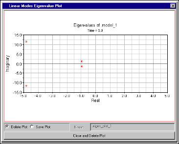
Figure 6 Plot of Two-DOF Model Eigenvalues
The pair of values closest to the real axis corresponds to mode 1 and the other pair corresponds to mode 2.
2. Select Close and Delete Plot.
3. In the Linear Modes Control dialog box, select Table.
Two rows of data appear in the information window as shown in Figure 7.
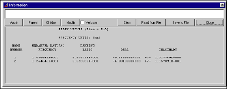
Figure 7 Table of Two-DOF Model Eigenvalues