FE PART Formulation
2D Beam
The 2D beam element is derived from the Absolute Nodal Coordinate Formulation (ANCF) Euler-Bernoulli beam theory[1-3]. These elements are ideally suited for long, slender beam with negligible shear deformation. The 2D beam element is a two-node beam element with a position vector and a gradient vector used as nodal coordinates  . Thus, each node has 4 coordinates: 2 components of the global position vector and 2 components of the position vector gradient at each node. This formulation displays no shear locking problems and it is computationally more efficient compared to the original ANCF due to the reduced number of nodal coordinates. It should be noted that these beam elements do not exhibit any out-of-plane motion and they should be defined in (and their motion is limited to) the plane parallel to the global XY, YZ or ZX plane.
. Thus, each node has 4 coordinates: 2 components of the global position vector and 2 components of the position vector gradient at each node. This formulation displays no shear locking problems and it is computationally more efficient compared to the original ANCF due to the reduced number of nodal coordinates. It should be noted that these beam elements do not exhibit any out-of-plane motion and they should be defined in (and their motion is limited to) the plane parallel to the global XY, YZ or ZX plane. The global position vector of an arbitrary point on the beam centerline with element spatial coordinate x is given by:
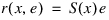
The shape function matrix for this element is defined as:
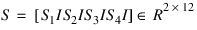
where:
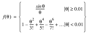
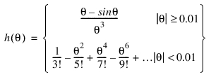
I is the  identity matrix and the shape functions Sj, j = 1,...,4 are defined as:
identity matrix and the shape functions Sj, j = 1,...,4 are defined as: 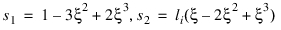
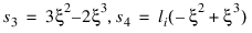
Here  is the length of the ith element, and
  is the vector of element nodal coordinates.
is the length of the ith element, and is the vector of element nodal coordinates.The mass matrix for the ith element is computed as:
where  and Ai are the mass density and the cross sectional area, respectively. One of the salient attributes of this formulation is that the mass matrix does not depend on the nodal coordinates and it remains constant during the simulation. The mass matrix is symmetric and consistent (not lumped).
and Ai are the mass density and the cross sectional area, respectively. One of the salient attributes of this formulation is that the mass matrix does not depend on the nodal coordinates and it remains constant during the simulation. The mass matrix is symmetric and consistent (not lumped). The external force vector ( ) for the ith element due to gravity can be obtained as:
) for the ith element due to gravity can be obtained as:
where  is the gravity force vector considering Y as the vertical axis.
is the gravity force vector considering Y as the vertical axis. The strain energy expression for the ith element is
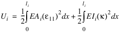
where 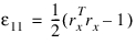 is the axial strain and
  is the magnitude of curvature vector. For initially curved beam (with no pre-stresses), the strain energy expression becomes
is the axial strain and is the magnitude of curvature vector. For initially curved beam (with no pre-stresses), the strain energy expression becomes 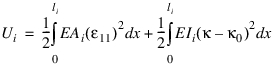
The elastic forces vector ( ) for the ith element is determined from the strain energy expression as
) for the ith element is determined from the strain energy expression as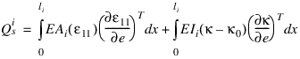
It should be noted that all the integral functions are computed numerically using the Gauss-quadrature formula. The nodal coordinate vector, the external and elastic force vectors, and the mass matrix for the entire beam are formed using the element connectivity.
3D Beam
The 3D beam formulation is derived from both the ANCF shear deformable beam theory and the geometrically exact beam formulation [4-7]. A beam is described by its centroid line r(x,t) and the cross section moving frame A(x,t), where A = [n t1 t2] is the transformation matrix from the moving frame to the global coordinate system.
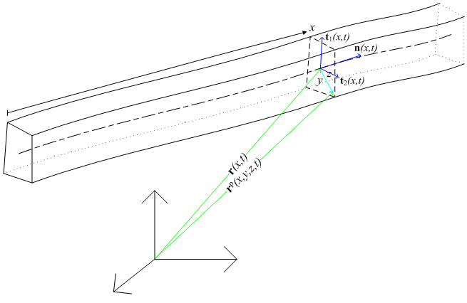
Figure 1 Geometrical description of a particle on the beam
As shown in Figure 1, the coordinates of a particle P on the beam are defined as
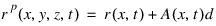
where d = (0 y z)T define the coordinates of particle in the cross section reference frame.
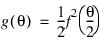
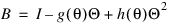
The transformation matrix A(x,t) is described by the rotation vector  , which is
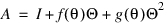
, which is where I is the  identity matrix;
 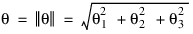 ; and
; and
identity matrix; ; and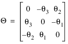 ,
,  ,
, 
The position vectors of the centroid line  and the rotation vectors of the moving frames
  are independently interpolated in each element
and the rotation vectors of the moving frames are independently interpolated in each element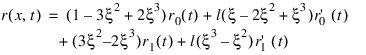

where l is the length of the element,  is the normalized arc-length coordinate in the element.
is the normalized arc-length coordinate in the element.
Figure 2 Generalized coordinates of 3D beam element
As shown in Figure 2, the generalized coordinates of a beam element are
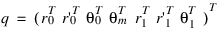
Thus, each 3D beam element has 21 generalized coordinates. The governing equation of the beam can be derived from Lagrange's equation
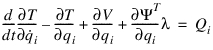

where
T = the total kinetic energy of the beam
V = the total elastic potential energy of the beam
 = the constraint equations
 = the Lagrange multipliers for the constraints
Q = the generalized applied forces
The kinetic energy of the kth element is
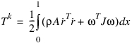
where

in which
with
and
 = density of the beam
A = area of the cross section
J = rotary inertia of the cross section
 = angular velocity of the moving frame
The elastic potential energy of the kth element is
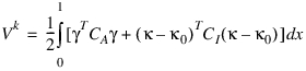
where
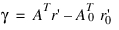 ,
, 
 = strains of the centroid line
 = curvature of the moving frame
(.) = the corresponding value in the un-deformed configuration
CA = stiffness matrix of the strain
CI = stiffness matrix of the curvatures
in which
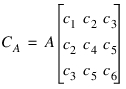 ,
,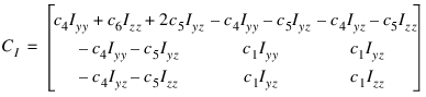
with
 ,
, ,
,
For isotropic materials, c1 = E, c4 = c6 = G, and c2 = c3 = c5 = 0.
For orthotropic materials, c1 = Ex , c4 = Gxy, c6 = Gxz, and c2 = c3 = c5 = 0.
The virtual work done by the external force in the kth element is
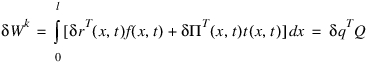
where
■
■f = applied distributed force on the beam
■t = applied distributed torque on the beam