Steps for Running Example
1. Ensure you have an installation of Actran 2020 SP1 or later.
2. Copy the tutorial directory included with the installation from "<top_dir>\acoustics\examples\tutorial\cooler_basic\" to some location on your machine you are comfortable using as a working directory.
Note: | "top_dir" is the path in which Adams was installed) |
3. Launch Adams View, choose to open an existing model and browse for cooler_ws.cmd in the directory to which you copied it.
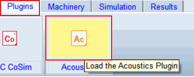
4. On the Plugins tab of the ribbon inside the Acoustics container, click the Actran logo to load the plugin:
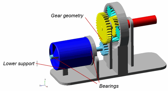
5. The model should now be open in the Adams View session. Familiarize yourself with it. A torque is applied to the input shaft, which starts to spin up the rotor shaft of the cooler.
6. Simulate the Adams model:
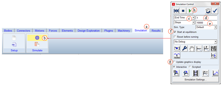
a. Go to the ribbon tab Simulation
b. From the options available select "Run an Interactive Simulation"
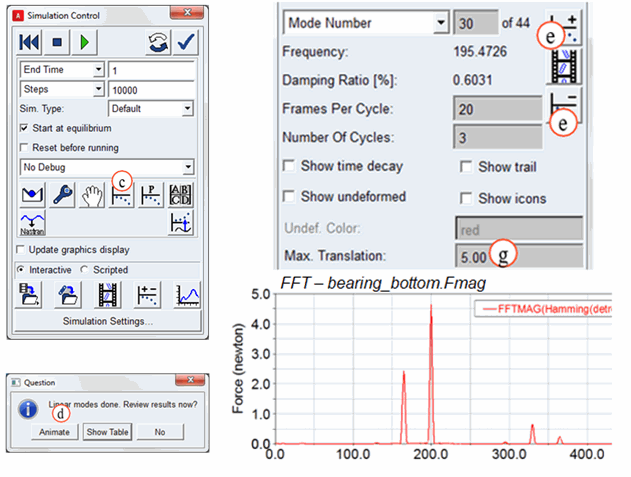
c. In the Simulation Control dialog box select End Time
d. In the text box adjacent to End Time, enter 1
e. In the text box adjacent to Steps enter 10000
f. Select Start at equilibrium
g. Do not update graphics display during simulation
h. Click on the Play tool to start the simulation
i. When complete close the Simulation Control dialog box
7. Animate Adams Results
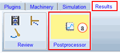
a. Select the ribbon tab Results and open Adams PostProcessor
b. In Adams PostProcessor, select Animation from the drop-down option menu
c. Right-click in the window and select to Load Animation
d. Before you start the animation, select to animate only every 5th frame (Frame Increment=5)
e. Start the animation using the play button
f. Rotate the view using the keyboard shortcut "r" if you like
g. Try also to animate only the last 0.1sec, to see the steady-state condition:
♦Start = 9000
♦Frame Increment=1
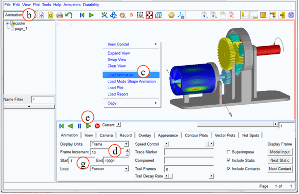
Note how the bearing forces change due to the gears, and how the housing starts to vibrate.
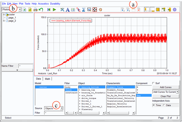
8. Plot some results:
a. Open a new page in Adams PostProcessor
b. Select Plotting from the drop-down menu
c. Select to plot some results, for example:
♦Bearing forces (use Source=Objects)
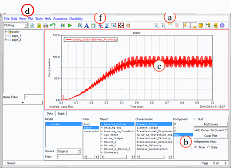
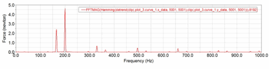
9. Do an FFT on the bearing force signal
a. Open a new page in Adams PostProcessor
b. Plot the magnitude of the force "bearing_bottom"
c. Click on the curve to select it
d. From the menu, select Plot - FFT
e. Enter time range 0.5-1.0, and Detrend Input Data
f. Note the major peak frequencies:_________Hz
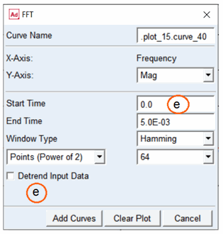
Hint: | To zoom in the FFT plot: Select the horizontal axis and unselect Auto Scale. Limits = 0 - 1000 Hz. 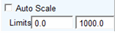 |
10. Run Actran Analysis
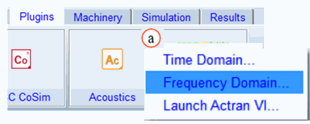
a. From the Plugins tab, select Acoustics - Frequency Domain
b. Right-click and select the flexible body "cooler_housing"
c. Click on Advanced Setup and go to the Mesh tab. Make sure Mesh Type is set to Automatic mesh. This means that Actran will create the acoustic mesh
d. Click on Create to create the skin mesh, shrinkwrap mesh
e. Click on Show to visualize the created meshes and the microphones' positions
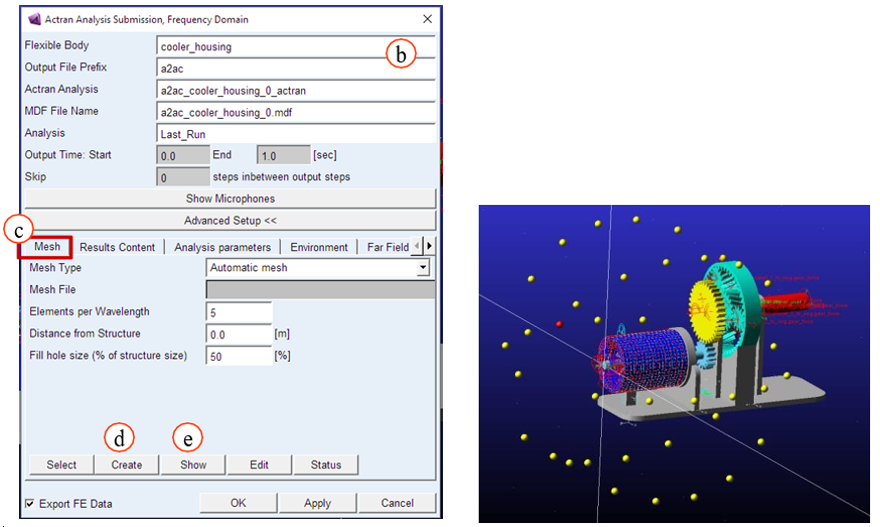
Note: | In the Frequency Domain acoustic simulations, only the shrinkwrap mesh around the flexible body is required at this stage. The volume mesh is created during the analysis and adapted by frequency band |
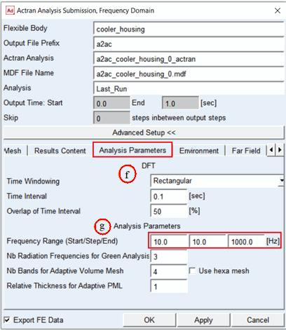
f. Go to Analysis parameters tab. Set the parameters as shown below. The DFT parameters section allows you to define the parameters of the Fourier Transform to switch from time domain Adams simulation to frequency domain simulation in Actran
g. The Analysis parameters section defines specific parameters of the Actran analysis. Details about these parameters are available in the documentation F1 Help. For the purpose of this excercise, you can limit the computation time by selecting a lower maximum frequency (1000Hz instead of 5000Hz proposed automatically)
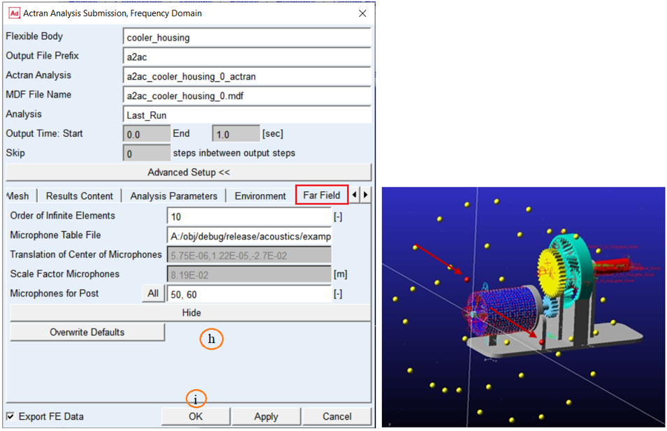
h. Go to the Far Field tab. Choose the parameters as shown below. For additional output set Microphones for post = 50, 60
i. Click on OK to run the Actran job analysis.
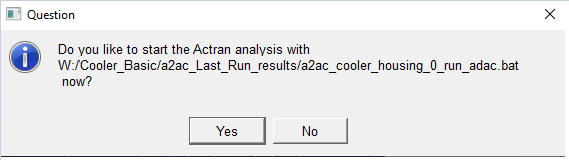
j. Choose Yes to start Actran analysis
■You can select No if you want to edit the parameter file (a2ac_cooler_housing_0_actran.par) and submit the analysis manually.
What happens now:

■The modal coordinates of the flexible body are exported from Adams on Nastran format (MDF). The modal coordinates are the scale factors of each mode that defines the elasticity of the flexible body in Adams.
■The modal coordinates are transformed into frequency domain by interval of 0.1s to take into account the evolution of the vibration over time.
■Actran starts to do a modal recovery of the housing part. The modal coordinates in frequency domain are combined with the modes of the flexible body to recover the motion of each node of the outer skin of the housing part.
■A frequency acoustic analysis is done, sound pressure levels at the
■microphone locations 50 and 60 are calculated.
■You can follow the progress of the Actran analysis in the log file: "a2ac_cooler_housing_0_actran_pre.log"
11. Results are stored in the working directory in a new directory called 'a2ac_Last_Run_results_xx'. A new sub-directory is created at every new Acoustics run in the working directory. 'xx' is the index of the simulation.

a. ACTAN_ANALYSIS contains the Actran input files and a plot config file (PLT file)
b. ACTRAN_POST_FREQ contains the specific outputs asked for by user (pictures and TXT files):
♦Sound Pressure Level (SPL) at microphones locations
♦Sound Power Level (SWL)
c. FE_Data contains the input data used for the calculation, especially the input structure mesh (BDF) and modes (MNF) of the flexible body. Hence all input data can be retrieved later
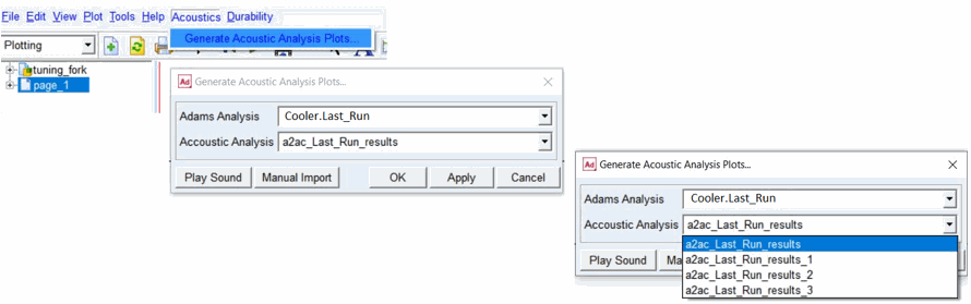
12. From the Acoustics menu select Generate Acoustic Analysis Plot and choose the Adams analysis and Acoustics analysis run in this exercise and click OK. This will generate several plots. See the documentation for more details about them.
a. Note that it is posisble to run multiple acoustics analyses per a single Adams analysis as illustrated below
b. The Manual Import button can be used to import acoustics results manually (for example, if you have results from an Acoustics toolkit installation that pre-date the product plugin release)
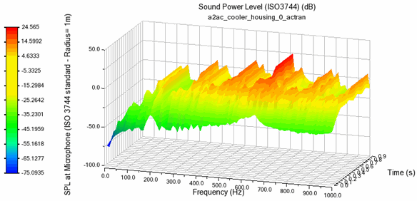
13. Auto-Plotted Results:
a. Sound power level in a 3D plot
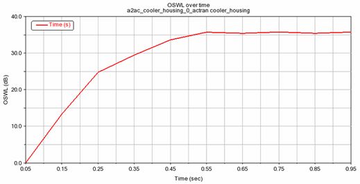
b. Overall sound power level
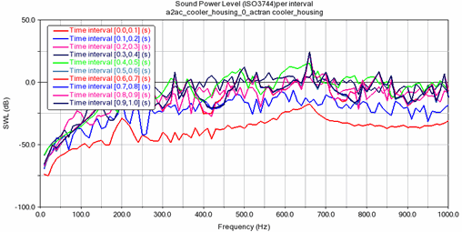
c. Sound power level at each time interval
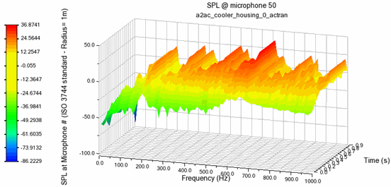
d. Sound pressure level at microphone
e. Sound pressure level per interval at microphone
f. Mean pressure
g. Overall sound pressure level
a. Sound power level at microphone
b. Overall Sound power level
c. Sound power level per time interval
d. Sound pressure level at microphone
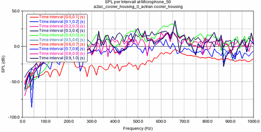
e. Sound pressure level per interval
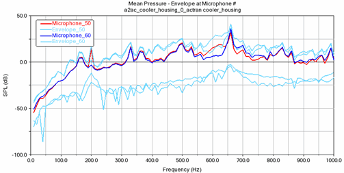
f. Mean pressure at microphone
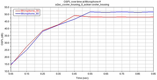
g. Overall sound pressure level
Optional Tasks
14. Linearize the Adams Model
A linearization of the Adams model will give us the eigen-modes and eigen-frequencies of the system. This is very useful information for understanding the frequency content of the model, and to better understand what modifications that may be useful to do to change the behavior of the system.
a. Run a new Adams time-domain dynamic simulation, as described in step 6
b. Do not close the Simulation Control dialog box
c. Click on the Linearize button
d. Select to animate the results
e. Click through the system eigen-modes, note the frequency and the shape
f. Try to find the system modes that contributed to the peak frequencies in the bearing load FFT you did earlier
g. You can change the mode deformation scale to better visualize it, if needed
15. Modify the model and try to improve (lower) the generated noise.
■Compare for example the sound power level between your iterations
■Model modifications of interest may be to:
a. Remove lower support of the housing
b. Change gear geometry (number of teeth, tip relief)
c. Modify bearing stiffness
d. Run analysis