Step Three - Adding Controls to the Adams Block Diagram
You will add controls to the Adams block diagrams by:
Starting MATLAB
A note about your Adams license(s): Running an Adams Controls cosimulation will check out an Adams Solver license and possibly an Adams View license (for interactive simulations only). To ensure that you are able to run these products, you may need to close any Adams applications that use these licenses.
To start using MATLAB:
1. Start MATLAB on your system.
2. Change directories to the one in which your ant_test.m file resides (the working directory you specified during your Adams Controls session).
You can do this by entering the following:
■On Windows: cd c:\new_dir, where new_dir is the name of your working directory.
■On Linux, cd /new_dir, where new_dir is the name of your working directory.
3. At the prompt (>>), type ant_test.
MATLAB echoes:
%%%INFO:Adams plant actuators names:
1 control_torque
%%%INFO:Adams plant sensors names:
1 rotor_velocity
2 azimuth_position.
1 control_torque
%%%INFO:Adams plant sensors names:
1 rotor_velocity
2 azimuth_position.
4. At the prompt, type who to get the list of variables defined in the files.
MATLAB echoes the following relevant information:
ADAMS_communication_interval | ADAMS_communications_per_output_step | ADAMS_cwd |
ADAMS_exec | ADAMS_host | ADAMS_init |
ADAMS_inputs | ADAMS_mode | ADAMS_outputs |
ADAMS_pinput | ADAMS_poutput | ADAMS_prefix |
ADAMS_solver_type | ADAMS_static | ADAMS_sysdir |
ADAMS_time_offset | ADAMS_uy_ids | ADAMS_version |
You can check any of the above variables by entering them in at the MATLAB prompt. For example, if you enter ADAMS_outputs, MATLAB displays all of the outputs defined for your mechanism:
ADAMS_outputs=
rotor_velocity!azimuth_position
Notes: | If you want to import the linearized Adams model, use ant_test_l.m instead of ant_test.m. The main difference is in the ADAMS_mode variable: ■In ant_test.m, ADAMS_mode=non_linear. ■In ant_test_l.m, ADAMS_mode=linear. |
Creating the Adams Block Diagram
To create the Adams block diagram:
1. At the MATLAB prompt, enter adams_sys.
This builds a new model in Simulink named adams_sys_.mdl. This model contains the Hexagon S-Function block representing your mechanical system.
A selection window containing the Adams blocks appears. These blocks represent your Adams model in different ways:
♦The S-Function represents the nonlinear Adams model.
♦The adams_sub contains the S-Function, but also creates several useful MATLAB variables.
♦The State-Space block represents a linearized Adams model.
Note: | An error or warning symbol may appear at the State-Space block indicating that the ADAMS_a, ADAMS_b, ADAMS_c and ADAMS_d variables do not exist in workspace. This is normal and can be ignored when the model has been exported as non-linear from the Adams controls plant export as in this example. |
The adams_sub block is created based on the information from the .m file (either from ant_test.m or ant_test_l.m). If the Adams_mode is nonlinear, the S-Function block is used in the adams_sub subsystem. Otherwise, the State_Space block is copied into adams_sub.
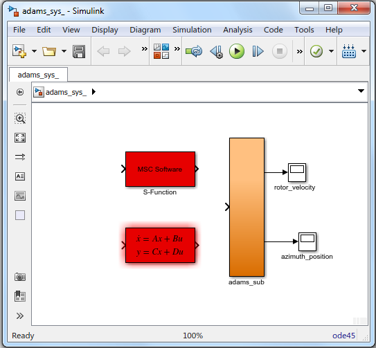
Figure 7 Simulink Selection Window
2. From the File menu, point to New, and then select Blank Model.
A new selection window for building your block diagram appears.
3. Drag and drop the adams_sub block from the adams_sys_ selection window onto the new selection window.
4. Double-click the adams_sub block.
All of the elements in the subsystem appear.
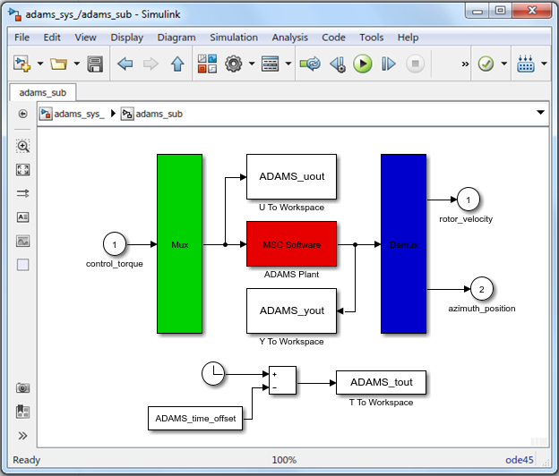
Figure 8 adams_sub block
Note: | The inputs and outputs you defined for the model appear in the sub-block. The input and output names automatically match up with the information read in from the ant_test.m file. |
Constructing the Controls System Block Diagram
The completed block diagram is in the file, antenna.mdl, in the examples directory. To save time, you can read in our diagram instead of building it. Remember to update the settings in the plant mask if you decide to use this file (see Setting Simulation Parameters in the Plant Mask).
Note: | If the Simulink model containing the adams_sub block was created in an earlier version of Adams Controls, you should run adams_sys again to create a new adams_sub block to replace the existing one for better performance. Only one adams_sub block is permitted per Simulink model. |
To construct the controls system block diagram:
1. At the MATLAB prompt, type simulink.
The Simulink library selection windows appear. Use the block icons from the windows to complete your controls block diagram. Each icon contains a submenu.
2. Double-click each icon to reveal its submenu.
3. Look at the controls block diagram Figure 9 and Table 1, which describes the topology in tabular form.
4. Drag and drop the appropriate blocks from the Simulink library to complete your block diagram as shown in Figure 9.
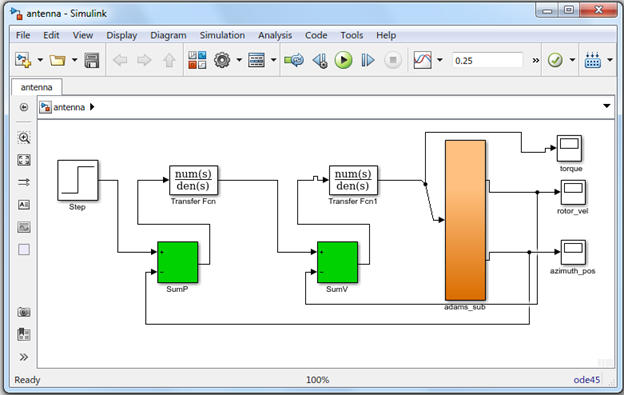
Figure 9 Controls Block Diagram
5. From the File menu, select Save As, and enter a file name for your controls block diagram.
Quantity | Library | Block Type | ||
1 | Sources | Step | ||
2 | Continuous | Transfer Function | ||
2 | Math Ops | Sum | ||
3 | Sinks | Scope(not floating) | ||
Step Parameters | Continuous Transfer Function Parameters | |||
Step Time: 0.001 | 1 | Numerator: [1040] | ||
Initial Value: 0 | Denominator: [0.001 1] | |||
Final value: 0.3 | Absolute tolerance: auto | |||
Sample time: 0.001 | 2 | Numerator: [950] | ||
[X] Interpret vector parameters as 1-D | Denominator: [0.001 1] | |||
[X] Enable zero crossing detection | Absolute tolerance: auto | |||
Sum Parameters | Scope | |||
1 | SumP | 1 | torque | |
Icon shape: rectangular | 2 | rotor_vel | ||
List of signs: +- | 3 | azimuth_pos | ||
[ ] Show additional parameters | ||||
2 | SumV | |||
Icon shape: rectangular | ||||
List of signs: +- | ||||
[ ] Show additional parameters | ||||
Setting Simulation Parameters in the Plant Mask
To set the simulation parameters:
1. From the controls block diagram, double-click the adams_sub block.
2. From the new Simulink selection window, double-click the Hexagon block.
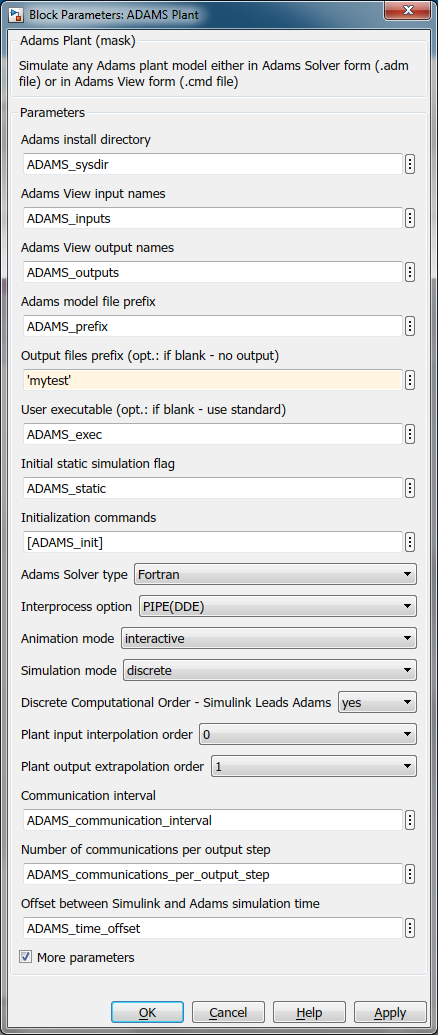
The Adams Plant Mask dialog box appears.
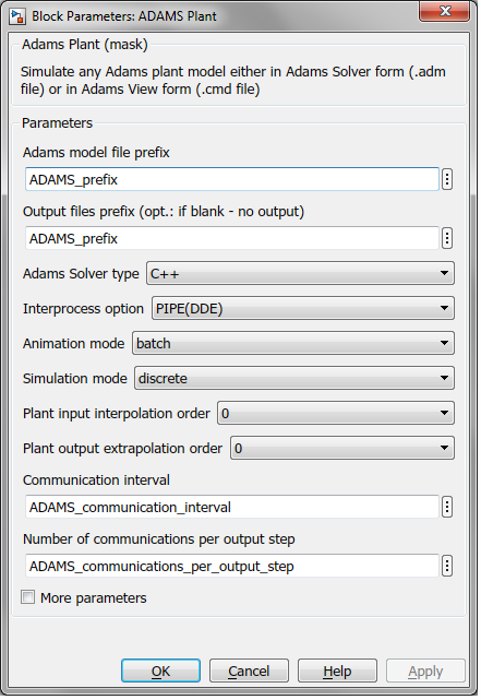
Figure 10 Adams Plant Mask
3. In the Output Files Prefix text box, enter ‘mytest’.
Be sure to enclose the name with single quotation marks. Adams Controls will save your simulation results under this name in the three file types listed in Table 2‑1
Note: | If no output files are required, then insert empty single quotes (''). |
File Name | File type: | What the file contains |
|---|---|---|
mytest.res | Results | Adams Solver analysis data and Adams View graphics data |
mytest.req | Requests | Adams Solver analysis data |
mytest.gra | Graphics | Adams View graphics data |
4. Select the Adams solver type of Fortran.
To run the simulation using Adams Solver (C++), you can change the setting to C++.
5. Select the Interprocess Option of PIPE(DDE).
This option defines the communication method between MATLAB and Adams. You can change this setting to TCP/IP, if you want to run MATLAB and Adams on separate machines and communicate using TCP/IP protocol. Using this protocol, Adams_host defines the machine on which Adams runs. For more information, see TCP/IP Communication Mode in the Adams Controls help.
6. Select a simulation parameter for each text box.
■Set Animation mode to interactive.
Animation mode controls whether you graphically monitor your simulation results in Adams View (interactive), or you simulate with Adams Solver (batch). See the online help for more details about animation modes.
■Set Simulation mode to discrete.
This mode specifies that the simulation run in co-simulation -- Adams solves the mechanical system equations and that the controls application solves the control system equations. The variables exchanged between Adams and MATLAB are exchanged at "discrete" intervals. See the online help for more details about simulation modes.
7. Keep the default Communication Interval parameterized, but change the variable value in the Workspace by executing the following command in the Matlab command window: ADAMS_communication_interval = 0.001
The communication interval defines how often the communication between Adams and Simulink occurs. This will affect simulation speed and accuracy.
8. Keep the default Number of communications per output step.
This value controls the size of .res, .req,and gra files. It must be an integer larger than zero. For example, if the value is n, Adams Controls writes to the output file once for every n communication steps. This size-control mechanism only works in discrete mode.
9. To save the change, select Apply.
10. Select Cancel to close the plant mask.
Note: | For more features in the Adams Controls block, select More parameters, which reveals the following dialog box. Note that the dialog box will add and remove parameters depending on the settings. |
This plant uses the following variables:
ADAMS_sysdir | Adams installation directory |
ADAMS_inputs | Input variables View names vector |
ADAMS_outputs | Outputs variables View names vector |
ADAMS_prefix | Adams model files prefix (.adm, .cmd); also doubles as output files prefix |
ADAMS_exec | Adams Solver user library or keyword (for example, acar_solver) |
ADAMS_static | yes|no - initial static before Co-simulation(discrete)/Function Evaluation (continuous) |
ADAMS_init | Initialization commands (that is, Adams View or Solver commands, depending on setting for Animation mode) |
ADAMS_cwd | Current working directory (for TCP/IP) |
ADAMS_host | Name of Adams server host (for TCP/IP) |
ADAMS_mode | Linear or non-linear (that is, co-sim, function eval) |
ADAMS_solver_type | FORTRAN or C++ (used to set popup menu when first loaded) |
ADAMS_communication_ interval | Time step at which Co-simulation exchange information (for example,0.005); also controls output for continuous mode (Function Evaluation) |
ADAMS_communications_ per_output_step | Sets Adams output rate (.res, .req, .gra) integer value (default: 1) |
ADAMS_time_offset | Adams uses the Simulink simulation time minus ADAMS_time_offset (default: 0.0). For example, if ADAMS_time_offset = 2, the Adams simulation starts (at Adams time = 0s) when the Simulink time = 2s. Make sure that the Adams block is disabled when the Adams time is <0s. If not an error will be raised. |
The following settings can be chosen:
Adams Solver type | FORTRAN or C++ (will also set ADAMS_solver_type) |
Interprocess option | Pipe (DDE), TCP/IP or DIRECT; TCP/IP can allow different machines run Adams and MATLAB. In DIRECT mode Adams runs as a library within MATLAB and no inter-process communication is involved. This mode requires MATLAB and Adams to run on the same PC. It works only when "Animation mode" is set to batch and "Adams Solver type" is set to C++. When running in Linux, this mode requires the user to be logged in as root. If the user uses a different login other than root, then the LD_LIBRARY_PATH environment variable has to be set explicitly to point to "<Adams install dir>/linux64" before starting MATLAB. For example, if Adams is installed at /scratch/Adams/20xx, then the environment variable should be set as below (This example assumes bash shell. For a different shell, use the appropriate format). export LD_LIBRARY_PATH=/scratch/Adams/20xx/linux64:$LD_LIBRARY_PATH In some scenarios on Linux, it has been observed that using DIRECT mode with MATLAB causes the MATLAB to hang or crash when the simulation is running or at the end of simulation. In such scenarios it is recommended to start MATLAB using the -nojvm option. This should cause the simulations to run properly. Alternately, the PIPE option could be used instead of DIRECT. |
Animation mode | batch (Solver, uses .adm) or interactive (View, uses .cmd) |
Simulation mode | discrete (Co-simulation) or continuous (Function Evaluation) |
Discrete Computational Order - Simulink Lead Adams | For discrete mode, chooses if Simulink leads the integration (yes) or lags (no); if set to no, can remove algebraic loop |
Plant input interpolation order | 0 = zero-order hold; 1 = linear (discrete mode only, where Simulink leads) |
Plant output extrapolation order | 0 = zero-order hold; 1 = linear (discrete mode only, where Simulink leads) |
Plant input extrapolation order | 0 = zero-order hold; 1 = linear (discrete mode only, where Adams leads) |
Plant output interpolation order | 0 = zero-order hold; 1 = linear (discrete mode only, where Adams leads) |
Direct feedthrough | yes|no - yes = Input directly effect output (continuous mode-only) |