Step Seven – Create GSE from the Simulink Model
First you will start Adams View and import the command file, and then simulate your Adams model containing the GSE for the control system.
To start Adams View and load the command file:
1. Launch Adams View and import the file ant_test.cmd.
2. Load the Adams Controls plugin, if not already loaded.
3. From the Plugins tab, click on the Controls container, point to Control System, and then select Import.
The Adams Controls System Import dialog box appears.
4. Select Import I/O Signals from Existing Controls Plant.
5. From the Database Navigator, select ant_test for the plant. The values for the Output Signals and Input Signals text boxes appear.
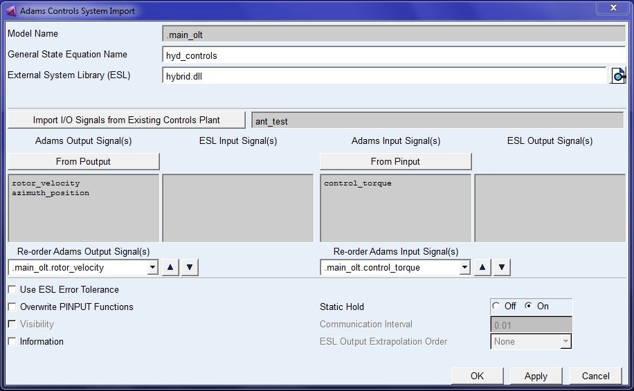
Figure 21 Adams Controls System Import Dialog Box
Adams View displays information on the GSE created (See Figure 22). The Database Navigator shown in Figure 23 shows the GSE and its associated arrays.
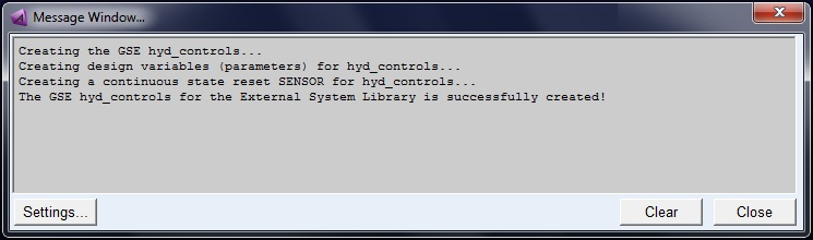
Figure 22 Information Window
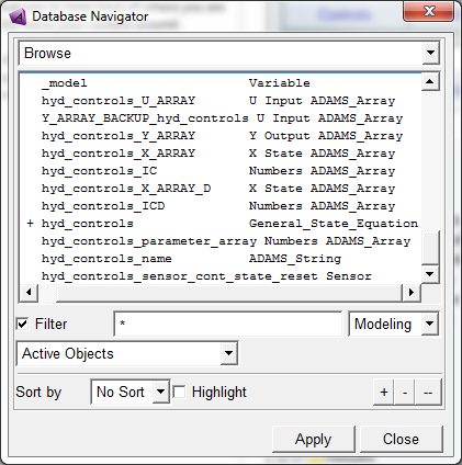
Figure 23 Database Navigator
To simulate your model:
1. From the Settings menu, point to Solver, and then select Dynamics.
The Solver Setting dialog box displays.
2. Change Formulation to SI2.
3. Set Category to Executable.
4. Set Hold License to No.
This setting is critical to using the RTW dll in repeated simulations in Adams View.
When you rewind/stop a simulation in Adams View, the RTW dll is released and reacquired, thereby resetting the discrete states and counters to their original state. Changing this behavior by issuing commands in Adams View causes unexpected simulations after the first one.
5. Select Close.
6. Run a simulation with a step size of .001s and duration of .25s.
During the simulation, the antenna motion behaves the same as the one in the co-simulation.
7. Press F8 to open Adams PostProcessor.
8. Plot and animate, as desired.
Adams PostProcessor displays the plot of azimuth position versus time, as shown in below figure.
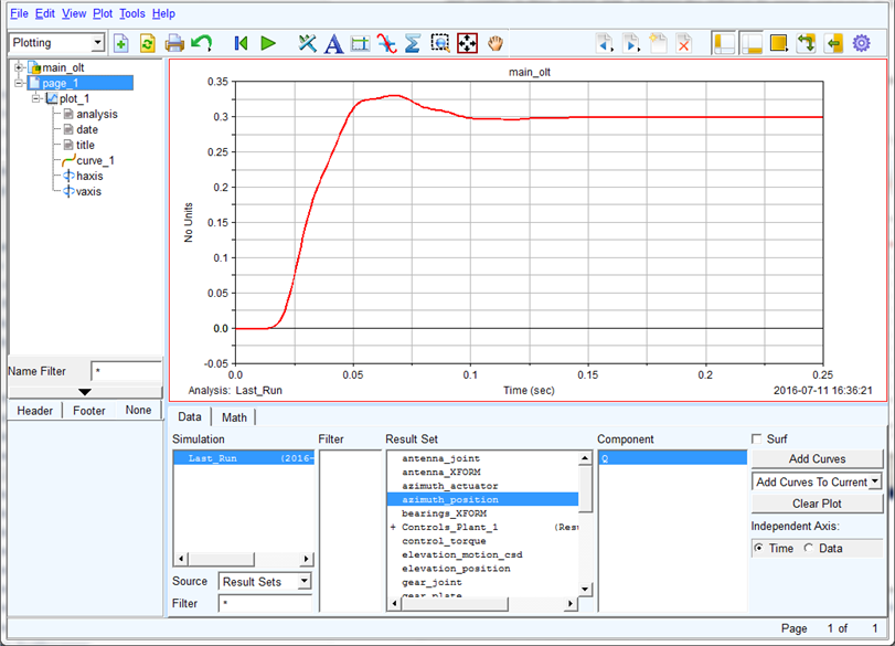
Figure 24 Plot of Azimuth Position vs. Time
A comparison of the results of the above simulation, Co-simulation, and Function Evaluation simulation is conducted (the latter two not performed in this tutorial). In all cases, the output step (sampling time in discrete simulation) is set to .01 second. The control torque versus time from three simulations is plotted in Figure 25. As shown, the result from the simulation with imported GSE is almost the same as that from Function Evaluation simulation. The control torque from the Co-simulation is slightly larger in magnitude because the one-step delay introduced by the discrete control system results in a control-mechanical system with less damping.
Your RTW dll can contain discrete states and counters. When performing repeated simulations (for example, design of experiments or design optimization), these entities need to be reset to their original values at the beginning of each simulation. When you rewind a simulation in Adams View, the RTW dll is released and reacquired, thereby resetting the discrete states and counters to their original state. Changing this behavior by issuing commands in Adams View causes unexpected simulations after the first one.
Figure 25 Control Torque vs. Time
Optionally, if you repeat the tutorial to create ESL's for discrete and continuous models, and re-run, you should see a plot like Figure 26. Note that the step excitation is slightly different for each model, and delays are caused by discrete states, so you should see differences in the responses accordingly.
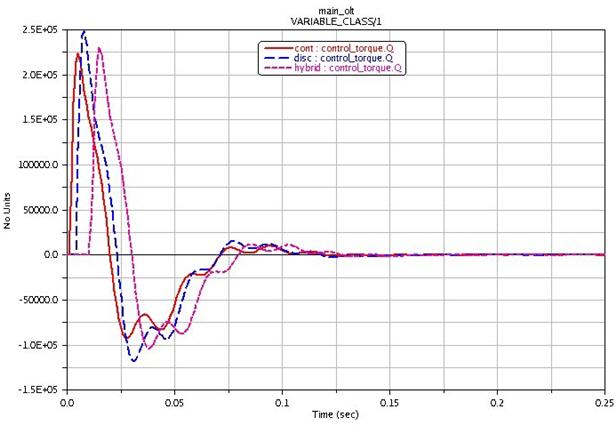
Figure 26 Re-run Result