Part 2 - System-Level Simulation
In this section, you will run a dynamic simulation of the vehicle to produce loads (modal coordinates) for the flexible lower control arm (LCA) in the left-front suspension. The modal coordinates will be exported to MSC.Fatigue and used for stress calculation.
In this session you will perform the following steps:
Importing the Model into Adams View
To import the model into Adams View:
1. Start Adams View.
2. In the Welcome dialog box, select Import a file.
3. Select OK.
4. In the File to Read text box, enter ATV_4poster.
There is no need to browse for this file. By typing in the name, Adams View locates the file in the Adams installation directory (in durability/examples/ATV).
5. Select OK.
This model contains the all-terrain vehicle standing on a four-poster rig. All parts are rigid.
Building the Flexible Suspension Arm
Next you will replace the rigid LCA with a flexible one.
To build the flexible suspension arm:
1. Zoom in on the left LCA in the front suspension as shown in the figure below.
Figure 3 Left LCA
■To rotate the view: Press r on the keyboard, and then rotate while pressing left mouse button.
■To translate: Press t.
■To zoom: Press w.
2. To replace the rigid LCA with a flexible LCA, from the Bodies tab, select the Flexible Bodies container, and then click the Rigid To Flex tool  .
.
. 3. In the Alignment tab, select the rigid part you want to replace and the MNF as follows:
■Current Part: RB2_left_lca_59
■MNF File: left_lca_0.mnf
■To select the rigid body to be replaced, right-click the Current Part text box, point to Part, and then select Pick. Using your mouse, click on the lower left suspension arm.
To browse for the MNF, right-click the MNF File text box, and then select Browse.
The flexible body defined in the .mnf is already correctly positioned so this is all you need to do in the Alignment tab.
4. Select the Connections tab.
The table displayed compares the connection points on the flexible body with the connection points on the rigid body. In the Distance column, you will notice that there is a small offset for the four bushing connection points.
You want to keep the bushings at the point where they where originally defined in the rigid model.
5. Click on the first table row, and then select Preserve location.
6. Repeat the previous step for rows 2 through 4 of the table.
The table should now look as shown in the figure below.
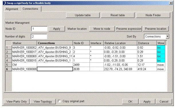
Figure 4 Connections Table
7. Select OK.
The rigid part is now replaced by the flexible body as defined in the .mnf. The flexible body is connected to the frame, knuckle, and damper in the same way as the rigid body.
To verify that the flexible LCA is correctly connected to the rest of the model:
1. From the Tools menu, select Database Navigator.
2. Select Topology By Parts.
3. Select the flexible LCA, .ATV_4poster.RB2_left_lca_59_flex.
It should be connected to the frame using two bushings, and to the damper (shock) and knuckle with one bushing each.
4. Close the Database Navigator.
Animating Modes of the Flexible LCA
To animate the modes of the flexible LCA:
1. Right-click the flexible LCA, and then select Modify.
2. Animate the modes by selecting a Mode Number (that is, 7) and then selecting the Animation tool  .
.
.You can animate each of the 40 modes calculated by MSC.Nastran and imported from the .mnf.
In the dynamic simulation results, expect to see 40 modal coordinates, one coordinate for each mode.
The first mode of interest is mode number 7. Modes 1 through 6 are rigid-body modes and are automatically disabled.
The first few modes are very similar to the free-free modes of the component. The high-frequency modes are usually unusual looking, but useful for describing local deformations around the attachment points.
Modifying the Damping of the Flexible LCA
The high-frequency modes are normally not very active in a dynamic simulation. There are two strategies to avoid them:
■Disable the modes. This may cause simulation difficulties if any of the disabled modes are necessary to describe, for example, a static position with local deformation around an attachment point.
■Modify damping so high-frequency modes are critically damped. The modes are enabled, but don’t participate in the dynamics because of the high damping applied to them.
Here, you will use the method of setting critical damping on the very high frequency modes. A STEP function will define the damping. The higher the frequency, the higher the damping.
To modify the damping of the flexible LCA:
1. If the Flexible Body Modify dialog box is not already displayed, right-click the flexible LCA, and then select Modify.
2. Clear the selection of default next to Damping Ratio.
3. Enter the following function for the Damping Ratio:
STEP(FXFREQ,1000,0.005,10000,1)
This means:
■Modes with a frequency below 1,000 Hz will have damping ratio of 0.5%.
■Modes with a frequency above 10,000 Hz will have damping ratio of 100%.
■Modes in the range of 1,000 - 10,000 Hz will be increasing with respect to their frequency based on the STEP function.
Note that default damping is usually not useful, especially not in this case. If you used default damping here, you would get a 10% damping ratio for mode 7, which is too much considering the component is made of steel.
4. Select OK to save all modification and close the Flexible Body Modify dialog box.
Running the Adams Dynamic Simulation
To run the Adams dynamic simulation:
1. Change your Adams Solver settings:
■From the Settings menu, point to Solver, and then select Executable.
■Set Choice to C++.
2. Modify Adams Solver dynamics parameters:
■Set Category to Dynamics.
■Set Formulation to SI2 and Error to 0.01.
The Stabilized Index-2 formulation enables the integrator to monitor the integration error of velocity variables and, therefore, renders highly accurate simulations. A positive side effect of the SI2 formulation is that the Jacobian matrix remains stable at small step sizes, which increases the stability and robustness of the corrector at small step sizes. We use the SI2 formulation here because high accuracy of the inputs to the fatigue analysis is crucial.
3. Close the Solver Settings dialog box.
4. From the Simulate menu, select Interactive Controls.
5. Perform the following:
■Set End time to 10 seconds
■Change list2+ to Step Size
■Set Step size to 0.01 seconds
■Select Start at equilibrium position. If you do not start from equilibrium, your results will contain initial transient vibrations, which is not preferred.
■To avoid the screen being updated at every output time step taken by the solver (therefore speeding up the solve time), clear the selection of Update graphics display.
6. Select the Play tool  to start the simulation.
to start the simulation.Each post that the vehicle is standing on will move in the vertical direction to simulate the vehicle running in rough terrain. This could also have been done by defining tire forces and a road profile.
The simulation will take a few minutes.
Viewing Adams Results
To view the Adams results:
1. From the Review menu, select Postprocessing.
2. In the upper left corner of Adams PostProcessor, use the pull-down menu to select Plotting.
3. In the dashboard (the lower section of the postprocessing window) select, for example, the following:
■Source: Objects
■Filter: force
■Object: BUSHING_9. This is the bushing connecting the LCA with the spring/damper
■Characteristic: Element_Force
■Component: Mag
4. Select Add Curves
The plot displays as shown next. This is the time history of force magnitude in the bushing between the flexible CLA and the shock.
Figure 5 Adams Results
Next, you will use Adams Durability to view the stress data.
5. Load the Adams Durability plugin using Tools Plugin Manager.
6. Load the animation, by right-clicking in the window, and then selecting Load Animation.
7. Before you start the animation:
■In the Contour Plots tab, set Contour Plot Type to Max Prin. Stress.
■In the Camera tab, set Follow Object to RB1_frame_57 (the frame). Lock the rotations.
■Zoom in on the flexible LCA and orient the display so that you are looking at the bottom surface of the LCA.
8. Animate by pressing the Play button.
9. Reset the animation.
10. To create a table that lists the three most critical areas of the LCA, from the Durability menu, select Hot Spots Table, and then specify the following:
■Body: RB2_left_lca_59_flex (right-click in text box, point to body, and then select Pick or Browse)
■Analysis: Last_Run (right-click in the text box, point to Analysis, point to Guesses, and then select Last_Run)
■Type: Maximum Principal Stress
■Radius: 30.0
■Count: 3
11. Select Report.
When the calculation is complete, Adams Durability displays the Hot Spots table as shown in the following figure. The hottest spot is located around node 2990, which is located on the bottom surface of the LCA, close to the cross-beam connection.
12. Close the Hot Spots Information dialog box.
Figure 6 Hot Spots Table
Exporting Results to MSC.Fatigue
When you export the results to MSC.Fatigue, it is actually not the stresses as calculated in Adams that we export, it is only the modal coordinates that are exported. The stress shapes are already calculated (Part 1 - Mode-Shape Analysis) and stored in the XDB file. The stress shapes in the XDB file will be combined with the modal coordinates from Adams in MSC.Fatigue.
To export results to MSC.Fatigue:
1. From the Durability menu, point to MSC.Fatigue, and then select Export. Specify the parameters as follows:
■Flexible Body: RB2_left_lca_59_flex
■Job Name: ATV_4poster
■Modal Coordinates (make sure this box is checked)
■Analysis: Last_Run
2. Clear the selection of Run MSC.Fatigue.
3. Select OK.
Modal coordinates for the flexible LCA are now exported in DAC format (40 files with prefix ATV_4poster) suitable for import to MSC.Fatigue. One file is produced for each modal coordinate.