Part 3 - Fatigue Life Calculation
For this portion of the tutorial, you will use MSC.Fatigue as a plugin to Patran. There is also a stand-alone version of MSC.Fatigue that is offered with a limited version of Patran.
In this section, you will predict fatigue life to failure and life factor of safety based on modal superposition and a standard S-N analysis (also known as Stress Life or Total Life).
You will perform the following steps:
Setting up Stress-Life Analysis in MSC.Fatigue
To set up stress-life analysis in MSC.Fatigue:
1. Start Patran, and from the File menu, select Open to open the tutorial.db file that was created in Part 1 - Mode-Shape Analysis of this tutorial.
2. From the Tools menu, select MSC.Fatigue.
3. Select Main interface.
4. Complete the dialog box as shown next, being sure to set Analysis to S-N
.
5. Enter fat_left_lca for the jobname for the fatigue jobs in Patran. All fatigue-related files will have this prefix.
The bottom section of the MSC.Fatigue dialog box contains the five steps to complete your fatigue job:
■Three inputs - Solution Parameters, Material, and Loading
■Job control - Used to submit and monitor fatigue jobs
■Results - Used to postprocess fatigue results
6. Select Solution Params and complete the dialog box as shown next
:
The Certainty of survival is set to 99%, indicating the highest conservatism in material properties scatter.
The design life is the number of repetitions this part is expected to withstand without failure. MSC.Fatigue will perform an additional analysis to assess the load scaling factor to reach a given target life. A design life of 60000 is derived from a simple assumption that under the given loading condition, the target life is around 10,000 km and that the 10-second repetition was performed at an average speed of 60 km/h.
7. Select OK to close the Solution Parameters dialog box.
8. Select Material Info.
MSC.Fatigue offers a built-in library with more than 200 predefined materials. You can select multiple materials for the same run and access advanced material options, such as temperature dependency.
9. Click in the first cell of the spreadsheet (Material) and scroll through the available material list below it. Select MANTEN_SN (carbon wrought steel).
10. Select No Finish and No Treatment.
11. Set Region to Membrane.
The region is the part of your model that will be analyzed. As mentioned previously, you are only interested in the surface element and you will use the previously created Membrane group as the target region.
12. Keep the defaults for all remaining fields, and then select OK.
Importing and Combining Modal Coordinates in MSC.Fatigue
The Loading Information dialog box is the spreadsheet that displays the association between modal stresses (MSC.Nastran output) and modal coordinates (from Adams). This is the key in recreating the stress history at each node that will be used for rainflow cycle counting (central to fatigue analysis algorithm).
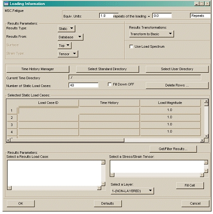
Figure 7 Loading Information Dialog Box
To import and combine the modal coordinates:
1. Select Loading Info.
To access the modal variables, MSC.Fatigue needs to load the relative *.dac files (the output from Adams created in Part 2 - System-Level Simulation) into the local time database (ptime.tdb).
2. Select Time History Manager to open the local time database. Then, perform the following:
■Select Load files.
■Select OK.
3. In the PTIME – Load Time History dialog box, enter the following:
■Source and target Filename: ATV_4poster*
■Description 1: modal coordinates
■Load Type: Scalar
■Units: none
■Select OK.
■The 40 files start loading. Select More enough times to make sure all load channels are loaded.
4. Select End.
The PTIME dialog box shows that you have 40 .dac files.
5. Select exit, and then select OK to close the PTIME-Database Options dialog box.
6. In the Loading Information dialog box, perform the following:
■Set Number of Static Load Cases to 40. Be sure to select Enter on your keyborard after setting this value. Doing so will update the number of rows in the spreadsheet from 1 to 40.
■Select Fill Down OFF and the option changes to Fill Down ON.
■Select the first cell in the Load Case ID column.
■Select Get/Filter Results to open the Results Filter dialog box.
■To access all available results in the database in the Results Filter dialog box, select Select All Results Cases, and then select Apply.
7. Select the first available results loadcase (… Mode 1…) in the Select a Results Load Case list.
8. From the Select a Stress/Strain Tensor list, select 1.1 – Stress tensor.
9. Select Fill Cell to populate the Load Case ID column.
10. Make sure the first cell in the Time History column is selected to populate column 2.
11. Select ATV_4POSTER_01.DAC from the Select a Time History list.
Your spreadsheet should look similar to the image shown below.
12. Leave the remaining default values, and then select OK.
Figure 8 Spreadsheet for ATV_4POSTER_01.DAC:
Running S-N Fatigue and Factor of Safety (FOS) Analysis
To run the analysis:
1. From the MSC.Fatigue menu, select Job Control.
2. To start the analysis, select Apply.
Wait a minute or two until the fat_left_lca fatigue job has been submitted.
You can check the status by accessing Job Control → Action → Monitor Job, and then periodically selecting Apply.
When completed, the status window displays the following message:
Safety factor analysis completed successfully.
If you receive the message ERROR: cannot communicate with Queue Manager, Patran is trying to run MSC.Fatigue through the Analysis Manager without a defined environment. A workaround is to deactivate the Analysis Manager using the Patran command analysis_manager.disable(), and then resubmit the job.
Importing and Reviewing Results in Patran
To import and review the results in Patran:
1. Select the MSC.Fatigue tab near the bottom right corner of the Patran window.
2. Select Results.
3. Select Apply to read in the results.
MSC.Fatigue automatically accesses the results based on the current job name.
The results are now stored in the Patran database as the Total Life and Factor of Safety subcases for postprocessing.
4. To view a quick plot of the factor of safety in Patran, select Results on the main Patran form (not in MSC.Fatigue).
5. In the results window, scroll through the list of Result Cases, and then select Factor of Safety, fat_left….
6. Select Safety Factor as the fringe result, and then select Apply.
The smallest factor of safety is 2.70. You can create a damage plot to improve the visualization of the critical areas.
To see a damage plot:
1. Select Total Life from the Result Cases list.
2. Select Damage from the Fringe Result list.
3. Select Apply.
Note that the highest damage occurs at three critical regions of the LCA.
Importing and Reviewing Results in Adams (Optional)
To import and review the results in Adams:
1. Click the Plugins tab on the Adams View ribbon.
2. From the Durability container, click Durability tool  and select MSC.Fatigue → Import.
and select MSC.Fatigue → Import. 3. Browse to the fatigue results file (*.fef), for example, ...\fat_left_lca.fef.
4. Select RB2_left_lca_59_flx as the flex body, and then select OK.
5. Select the Contour Plots tab.
6. Set Contour Plot Type to Life (Log Repeats).
The results are displayed in Adams PostProcessor, as shown below.
Because the results represent the total results for the simulation, you do not need to animate the results.
Figure 9 RB2_left_lca_59_flx Contour Plot