Evaluate the Fixed Step Integrator
1. The files required for this tutorial can be found in the Adams installation at: \install_dir\realtime\. Copy them to your working directory.
2. Start Adams Car (Standard Interface).
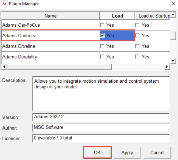
3. Load the Adams Controls plugin by clicking on Tools → Plugin Manager and set the corresponding check-box to Yes and click OK.
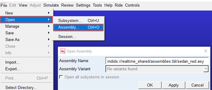
4. The realtime_shared.cdb database contains the following full-vehicle assembly:
sedan_rwd.asy: vehicle model with compliance double wishbone front and rear wheel suspensions. The PAC2002 transient tire model is used for the tires.
Open this assembly.
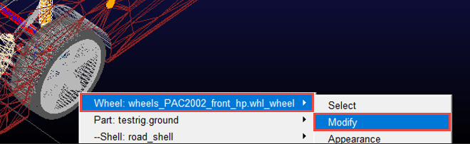
5. First, a simulation will be carried out with the default parameters of this model (GSTIFF, I3). To do this switch off the High Performance mode of the tires, by a Right Click (on the tires) → Wheel: wheels_PAC2002_front_hp.whl_wheel and select Modify.
In the Modify Wheel window, set the High Performance option to No, for both front and rear tires.
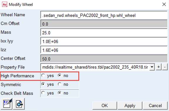
Note: | High Performance mode will improve the calculation performance of the PAC2002 model, but it needs a small solver time step (< 0.005 sec). |
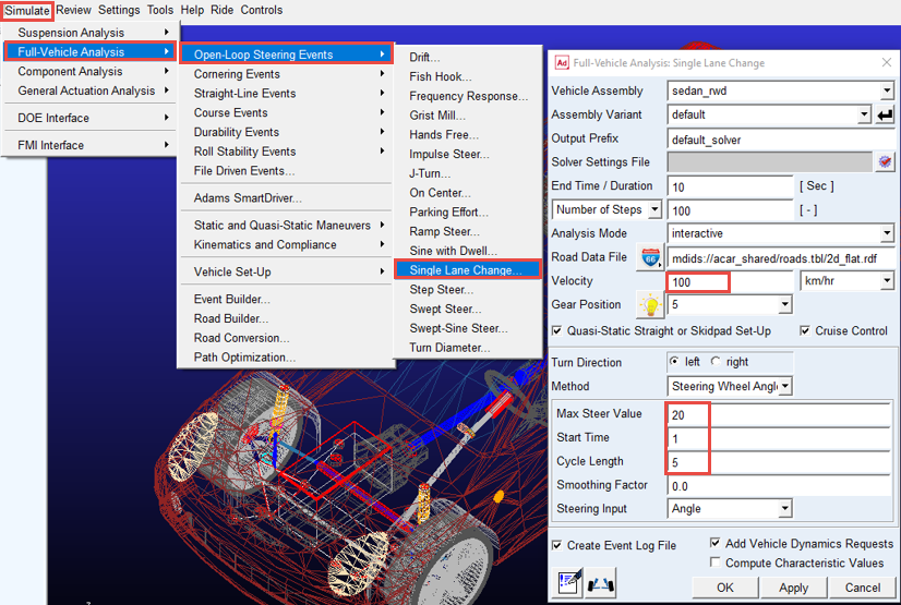
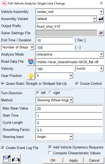
6. Now using the default Adams Solver settings, perform a single lane change maneuver: select Simulate → Full-Vehicle Analysis → Open Loop Steering Events → Single Lane Change, complete the dialog as shown below and click OK to run the simulation.
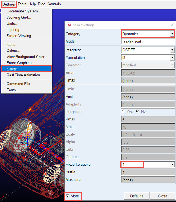
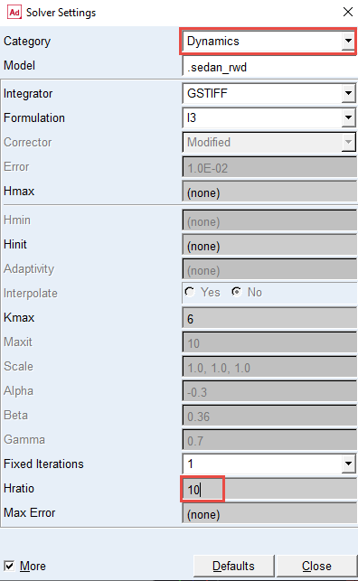
7. Next, set the GSTIFF integrator to use the fixed step option: select Settings → Solver and define values as follows:
♦Category: Dynamics and toggle More option.
♦Fixed Iterations: 1.
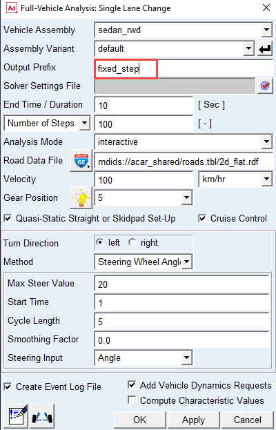
8. Re-run the same event this time with a different Output Prefix.
Note: | The simulation will not run due to singularities. This is due to the course step size, with the fixed step solver method: the step size method does not allow the Adams Solver to decrease step size when stability is a problem. 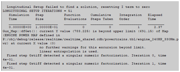 |
9. The solver step size can be adjusted by modifying the Hratio parameter. This parameter specifies the number of solver steps within one simulation interval. If Hratio is set to 10, the step size will be 0.001 sec with 0.01 interval step size:
To change the Hratio go to Settings → Solver and under the Dynamics Category set Hratio to 10.
To change the Hratio go to Settings → Solver and under the Dynamics Category set Hratio to 10.
Adjust the solver settings, and run the following simulation:
10. Make comparative plots of both analyses for vehicle motion and tire forces; you will notice a good agreement in between the simulation with and without fixed step method.
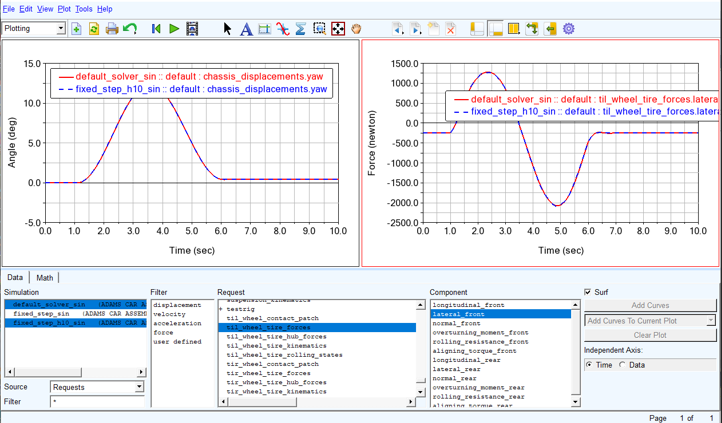
When checking the CPU and Elapsed time in the message files for the default_solver and fixed_step_h10 simulation, there is a large difference:
The ‘default_solver’ simulation lists in the .msg file (at a specific or linux windows platform):
Elapsed time = 27.54s, CPU time = 28.50s, Average CPU load = 103.49%.
While the ‘fixed_step_h10’ simulation shows at the same platform:
Elapsed time = 8.57s, CPU time = 9.38s, Average CPU load = 109.38%.
Naturally, finding the balance of accuracy and performance is at the heart of most CAE endeavors and preparing an Adams model for a real time environment is no exception. If one was not satisfied with the results after increasing hratio (or unconvinced that the results were converged) they could increase the number of fixed iterations as well and compare results further.
To learn more about the fixed step integrator please see the "Fixed Step Integrator Option" section within the production documentation at the INTEGRATOR statement and command entries in the Adams Solver C++ online help.