INTEGRATOR
The INTEGRATOR statement lets you control the numerical integration of the equations of motion for a dynamic analysis. You should use the INTEGRATOR statement when the default values for the numerical solution parameters are not optimal for a particular simulation.
Format
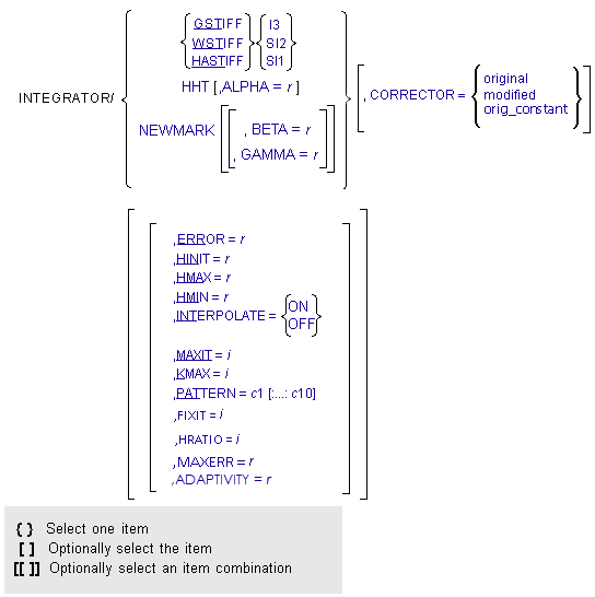
Arguments
ALPHA=r | Defining coefficient for the HHT method. Learn more about HHT. Default value: -0.3 Range: -0.333333 <= ALPHA <= 0 |
BETA=r | One of the two defining coefficients associated with the Newmark method. Default Value: 0.36 Range: Defined in conjunction with GAMMA. Together they must satisfy the stability condition.  |
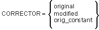 | Specifies the corrector algorithm that is to be used with the integrators. ■CORRECTOR=original - Specifies that the corrector available in the previous releases of Adams Solver (C++) be used. This is the default. This implementation of the corrector requires that at convergence, the error in all solution variables be less than the corrector error tolerance. ■CORRECTOR=modified - Specifies that a modified corrector is used. For GSTIFF, WSTIFF and HASTIFF, this implementation of the corrector requires that at convergence, the error in only those variables for which integration error is being monitored be less than the corrector error tolerance. This is a slightly looser definition of convergence, and you should use proper care when selecting this setting. For HHT and NEWMARK, this implementation of the corrector requires that the convergence assessment is to be performed ignoring fluctuations of the values in the Lagrange multipliers. ■CORRECTOR=orig_constant - Specifies that the original corrector is set and that no automatic switching to the modified corrector is to be performed. Adams Solver (C++) would switch from the original corrector to the modified corrector automatically under any of these two conditions: a. The model has CONTACT elements. By default, Adams Solver (C++) switches to the modified corrector when the model has CONTACT elements. b. There is an integration failure. In some cases, the integration algorithm will automatically switch to the modified corrector temporarily. When using the orig_constant option, Adams Solver (C++) will use the original corrector and no switching of the corrector algorithm is allowed. For additional information, see the Extended Definition. Default: corrector=original Note: Models containing CONTACT elements automatically switch to the modified formulation when Solver reads the model file. See Automatic corrector algorithm switches for more details. |
ERROR=r | Specifies the relative and absolute local integration error tolerances that the integrator must satisfy at each step. For BDF, HHT, and Newmark integrators, Adams Solver (C++) monitors the integration errors in the displacement and state variables that the other differential equations (DIFFs, LSEs, GSEs, and TFSISOs) define. The SI2 formulation also monitors errors in velocity variables. The larger the ERROR, the greater the error/step in your solution. Note that the value for ERROR is units-sensitive. For example, if a system is modeled in mm-kg-s units, the units of length must be in mm. Assuming that all the translational states are larger than 1 mm, setting ERROR=1E-3 implies that the integrator monitors all changes of the order of 1 micron. The error tolerance is compared against a local error measure that depends on the difference between the current predicted and corrected states, the past history of the states, and the current integration order. A slightly different integration ERROR definition is used for HHT and Newmark integrators. For these two integrators, the default is 1E-5. For more information, see Remarks. Defaults: ■HHT and Newmark: 1E-5 ■All other integrators: 1E-3 Range: ERROR > 0 |
FIXIT=i | Specifies 'fixed' number of corrector iterations to be taken per time step. Must be either unspecified or an integer from 1-10. If specified, the fixed step option is employed. If FIXIT is unspecified, then the fixed step option is not employed and Adams Solver integration proceeds in the traditional (that is, variable time step) manner. Default: unspecified Range: 1 < FIXIT < 10 |
GAMMA=r | One of the two (together with BETA) defining coefficients associated with the Newmark method. Default value: 0.7 Range: Defined in conjunction with BETA. Together they must satisfy the stability condition  |
GSTIFF | Specifies that the GSTIFF (Gear) integrator is to be used for integrating the differential equations of motion. |
HHT | Specifies that the HHT (Hilber-Hughes-Taylor) integrator is used for integrating the equations of motion. |
HINIT=r | Defines the initial time step that the integrator attempts. Default: 1/20 of the output step Range: 0 < HMIN < HINIT < HMAX |
HMAX=r | Defines the maximum time step that the integrator is allowed to take. Default: ■If INTERPOLATE = ON, the integration step size is limited to the value specified for HMAX. If HMAX is not defined, no limit is placed on the integration step size. ■If INTERPOLATE = OFF, the maximum step size is limited to the output step. Range: 0 < HMIN < HINIT < HMAX |
HMIN=r | Defines the minimum time step that the integrator is allowed to take. Default: ■1.0E-6*HMAX for GSTIFF, WSTIFF, and I3 ■Machine precision for GSTIFF, WSTIFF, SI2, and for HHT and Newmark Range: 0 < HMIN < HINIT < HMAX |
HRATIO=i | Specifies the 'fixed' ratio of the output sampling rate (aka "DTOUT") to the integrator time step size (aka "H"). Must be a positive integer. If unspecified while FIXIT is specified, this defaults to 1. HRATIO is only valid in the context of the fixed step option; so, it's ignored if FIXIT is unspecified. Default: 1 (with FIXIT on) Range: positive integer |
 | Specifies that the integrator is not required to control its step size to reach an output point. Therefore, when the integrator crosses an output point, it computes a preliminary solution by interpolating to the output point. Then, it refines (or reconciles) the solution to satisfy the equations of motion and constraint. Note that the IC statement/command defines the parameters controlling the reconciliation processes. (For example, position MAXIT, AERROR, and so on.) INTERPOLATE=OFF turns off interpolation for the chosen integrator. Default: OFF Note: When using INTERPOLATE with models containing CONTACT, you may see intermediate data at intervals that do not coincide with your specified output interval. This intermediate data (the data in-between the interpolated outputs) actually corresponds to contact incidences. You can turn off these extra contact data points with an environment variable, MDI_ADAMS_CONTACT_OUT. |
I3 | Specifies the Index-3 (I3) formulation be used. For more information, see Extended Definition. Default for GSTIFF/WSTIFF/HHT |
KMAX=i | Indicates the maximum order that the integrator can use. The order of integration refers to the order of the polynomials used in the solution. The integrator controls the order of the integration and the step size, and thus, controls the local integration error at each step so that it is less than the error tolerance specified. Note: ■For problems involving discontinuities, such as contacts, setting KMAX=2 can improve the speed of the solution. We do not recommend that you set the KMAX parameter unless you are a very experienced user. Any modification can adversely affect the integrators accuracy and robustness. ■KMAX is irrelevant (ignored) if the integrator selected is HHT or NEWMARK. Both these integrators are constant order (order 2 and 1, respectively) and therefore, the order does not change during simulation as is the case for the rest of the integrators available in the solver. Default: KMAX = 6 Range: 1 < KMAX < 6 |
MAXERR=r | Specifies the amount error above which the user would like the integrator to stop trying to solve the problem if it can't do better than this when the fixed step option is selected. If the local integration error exceeds MAXERR, the integrator stops the simulation. MAXERR is a positive real number. Similar to HRATIO, it's only relevant to the fixed step option; so, it's ignored if FIXIT is unspecified. When FIXIT is specified and this value is unspecified, then there is no amount of error which would cause Adams Solver to quit. Note that unlike ERROR, MAXERR does not control the accuracy of results. MAXERR can be interpreted as the pre-mature stopping criteria for simulation when the fixed step option is selected. Default: infinity Range: ERROR > 0 |
ADAPTIVITY=r | ADAPTIVITY modifies the integration error tolerance to include a term that is inversely proportional to the integration step size. This is intended to loosen the integration error tolerance when the step size gets small (i.e. integrator is struggling at the user-defined integration error tolerance). If the integration step size is equal to h, ADAPTIVITY/h is added to the integration error tolerance. Note: ADAPTIVITY has a different interpretation in FORTRAN Solver. ADAPTIVITY affects only the GSTIFF and HHT integrators in C++ Solver. In C++ Solver ADAPTIVITY is on by default and activated only when the integration step size is less than 100*HMIN. The default ADAPTIVITY in C++ Solver can be overridden when set to a real value, or it can be turned off by setting ADAPTIVITY=0 in the integrator statement/command. When using ADAPTIVITY, begin with a small number, such as ADAPTIVITY=1E-8. Note: This relaxes the integration error tolerance at small step size, which can introduce additional error into the dynamic solution. However, this can be beneficial for the models in which integrator struggles to satisfy the integration or corrector error. ADAPTIVITY is typically required to overcome integrator error difficulties or corrector convergence difficulties and you should not override its default setting in normal situations. If you use ADAPTIVITY in the integrator statement/command, be sure to validate your results by running another simulation using a different integration error tolerance. Default: depends on HMIN and ERROR settings Range: ADAPTIVITY > 0 |
MAXIT=i | Specifies the maximum number of iterations allowed for the Newton-Raphson iterations to converge to the solution of the corrector nonlinear equations. Typically, MAXIT should not be set larger than 10. This is because round-off errors start becoming large when a large number of iterations are taken. This can cause an error in the solution. Default: 10 Range: MAXIT > 0 |
NEWMARK | Specifies that the NEWMARK integrator be used for integrating the equations of motion. |
PATTERN=c1[:...:c10] | Indicates the pattern of trues and falses for reevaluating the Jacobian matrix for Newton-Raphson. A value of true (T) indicates that Adams Solver (C++) is evaluating a new Jacobian matrix for that iteration. A value of false (such as PATTERN=F) turns on the adaptive Jacobian evaluation algorithm. The evaluation of the integration Jacobian is then only done when needed. The algorithm determines a corrector convergence speed and based on this value, it extrapolates the configuration of the system after MAXIT iterations. The Jacobian is updated if the algorithm indicates that the convergence rate is too slow for the corrector to meet the convergence criteria. Overall, this approach is expected to result in fewer Jacobian evaluations, which in turn can lead to shorter simulation times. PATTERN accepts a sequence of at least one character string and not more than 10 character strings. Each string must be either TRUE or FALSE, which you can abbreviate with T or F. You must separate the strings with colons. Default: T:F:F:F:T:F:F:F:T:F (For GSTIFF and WSTIFF and for HHT/Newmark when FIXIT is specified) Default: F (For HHT/Newmark when FIXIT is not specified) Note: A pattern setting of all false implies that Adams Solver (C++) is to not evaluate the Jacobian until it encounters a corrector failure. For problems that are almost linear or are linear, this setting can improve simulation speed substantially. |
SI2 | Specifies that the Stabilized Index-2 (SI2) formulation, in conjunction with the GSTIFF, WSTIFF, or HASTIFF integrators, be used for integrating the equations of motion. The SI2 formulation takes into account constraint derivatives when solving for equations of motion. This process enables the GSTIFF and WSTIFF integrators to monitor the integration error of velocity variables, and, therefore, renders highly accurate simulations. A positive side effect of the SI2 formulation is that the Jacobian matrix remains stable at small step sizes, which in turn increases the stability and robustness of the corrector at small step sizes. The SI2 formulation is available only with GSTIFF, WSTIFF, and HASTIFF. For additional information, see the Extended Definition. |
WSTIFF | Specifies that the WSTIFF (Wielenga stiff) integrator be used for integrating the equations of motion. WSTIFF uses the BDF method that takes step sizes into account when calculating the coefficients for any particular integration order. Default: GSTIFF |
HASTIFF | Specify that the HASTIFF (Hiller Anantharaman stiff) integrator be used for integrating the differential equations of motion.HASTIFF uses the BDF method that takes step sizes into account when calculating the coefficients for any particular integration order. |
SI1 | Specifies that the Stabilized Index-1 (SI1) formulation, in conjunction with the HASTIFF integrator, be used for formulating and integrating differential equations of motion. The SI1 formulation takes into account constraint derivatives when solving for equations of motion. This process enables the HASTIFF integrator to monitor the integration error of velocity variables, and therefore renders highly accurate simulations. A positive side effect of the SI1 formulation is that the Jacobian matrix remains stable at small step sizes, which increases the stability and robustness of the corrector at small step sizes. The SI1 formulation is available only with HASTIFF, for which it is the default. |
Extended Definition
You use the INTEGRATOR statement to select an integrator when you choose to perform a dynamic analysis. The dynamic analysis of a mechanical system consists essentially of numerically integrating the nonlinear differential equations of motion.
Ordinary differential equations (ODEs) can be characterized as being stiff or non-stiff. A set of ODEs is said to be stiff when it has widely separated eigenvalues (low and high frequencies) with the high frequency eigenvalues being overdamped. Therefore, while the system has the ability to vibrate at high frequencies, it usually does not because of the associated high damping, which dissipates this mode of motion.
The stiffness ratio of a set of ODEs is defined as the highest inactive frequency divided by the highest active frequency. Stiff ODEs typically have a stiffness ratio of 200 or higher. In contrast, non-stiff systems have a stiffness ratio less than 20. This basically means that for a non-stiff system of ODEs, the higher frequencies of the system are active. The system can and does vibrate at these frequencies.
An example of a stiff system is a flexible body in which the higher frequencies have been damped out completely, leaving only the lower frequency vibration modes active.
The system above becomes non-stiff if the higher frequencies are excited by an external force. Nonlinear ODEs can be stiff at some points in time and non-stiff at other points.
Learn more about:
■SI2
Stiff and Non-Stiff Integrators
Integrators are classified as stiff or non-stiff. A stiff integrator is one that can handle numerically stiff systems efficiently. For stiff integrators, the integration step is limited by the inverse of the highest active frequency in the system. For non-stiff integrators, the integration step is limited by the inverse of the highest frequency (active or inactive) in the system. Thus, non-stiff integrators are notoriously inefficient for solving stiff problems.
Because many mechanical systems are numerically stiff, the default integrator in Adams Solver (C++) is GSTIFF, a stiff integrator that is based on the DIFSUB integrator developed by C.W. Gear. Gear's DIFSUB integrator is unrelated to the Adams Solver subroutine that is known by the same name. WSTIFF is another stiff integrator available in Adams Solver (C++). Both GSTIFF and WSTIFF integrators are based on Backward-Difference Formulae (BDF) and are multi-step integrators. The solution for these integrators occurs in two phases: a Prediction followed by a Correction.
Prediction
When taking a new step, the integrator fits a polynomial of a given order through the past values of each system state, and then extrapolates them to the current time to perform a prediction. Standard techniques like Taylor's series (GSTIFF) or Newton Divided Differences (WSTIFF) are used to perform the prediction.
Prediction is an explicit process in which only past values are considered, and is based on the premise that past values are a good indicator of the current values being computed. The predicted value does not guarantee that it will satisfy the equations of motion or constraint. It is simply an initial guess for starting the correction, which ensures that the governing equations are satisfied.
The degree of polynomial used for prediction is called the order of the predictor. For example, a predictor of order 3 will fit a cubic polynomial that includes the past 4 values for each state. Clearly, if the governing equations are smooth, the prediction will be quite accurate. On the other hand, if the governing equations are not smooth, the prediction can be quite inaccurate.
Correction
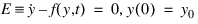
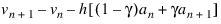
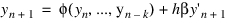
The corrector formulae are an implicit set of difference relationships (BDFs) that relate the derivative of the states at the current time to the values of the states themselves. This relationship transforms the nonlinear differential algebraic equations to a set of nonlinear, algebraic difference equations in the system states. The Backward Euler integrator is an example of a first-order BDF. Given a set of ODEs of the form dy/dt = f (y,t), the Backward Euler uses the difference relationship:
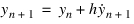 | (20) |
where:
■yn is the solution calculated at t = tn.
■h is the step size being attempted.
■yn+1 is the solution at = tn+1, which is being computed.
Notice that the subscript n+1 is on both sides of Equation (20). This is an implicit method.
Adams Solver (C++) uses an iterative, quasi-Newton-Raphson algorithm to solve the difference equations and obtain the values of the state variables. This algorithm ensures that the system states satisfy the equations of motion and constraint. The Newton-Raphson iterations require a matrix of the partial derivatives of the equations being solved with respect to the solution variables. This matrix, known as the Jacobian matrix, is used at each iteration to calculate the corrections to the states.
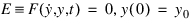
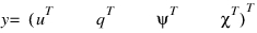
Assume that the equations of motion have the form:
 | (21) |
where y represents all the states of the system.
 and
and  gives:
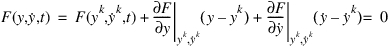
replacing y - yk with  and
and  with
with  , you get:
and with , you get: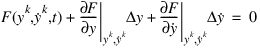 | (22) |
From Equation (20), which is a first-order BDF, you can get the relationship:
 | (23) |
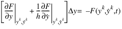 | (24) |
A generalization of (24)to higher-order BDFs gives:
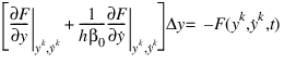 | (25) |
where:
■ is a scalar that is characteristic to an integration order. This scalar is constant for each integration order.
is a scalar that is characteristic to an integration order. This scalar is constant for each integration order. ■The matrix on the left side of Equation (25) is the Jacobian matrix of F.
■ are the corrections.
are the corrections. ■F is the residue of equations (equation imbalances).
The corrector is said to have converged when the residue F and the corrections  y have become small.
y have become small.After the corrector has converged to a solution, the integrator estimates the local integration error in the solution. This is usually a function of the difference between the predicted value and the corrected value, the step size, and the order of the integrator. If the estimated error is greater than the specified integration ERROR, the integrator rejects the solution and takes a smaller time step. If the estimated error is less than the specified local integration ERROR, the integrator accepts the solution and takes a new time step. The integrator repeats the prediction-correction-error estimation process until it reaches the time specified in the SIMULATE command.
Note: | The premise for using predictions as an initial guess for the corrector is severely violated when discontinuities occur or when large forces turn on or off in the model. Contact, friction, and state transitions (as in hydraulics where a valve is suddenly closed or opened) are examples of such phenomena. These kinds of models are difficult for multi-step integrators. |
The corrector in a stiff integrator ensures that all candidate solutions satisfy the equations of the system. The two algorithms, original and modified, differ primarily in the strategy that they use to define when the corrector iterations have converged.
The CORRECTOR=modified setting is helpful for models containing discontinuities in the forcing functions. Problems with contacts belong in this category.
Correction summary tables:
Error control in corrector:
Integrator and formulation | Original Corrector | Modified corrector |
|---|---|---|
GSTIFF I3, WSTIFF I3 | Error control on displacements, velocities of body equations, flex modes, flex mode velocities, applied forces, and state variables from differential equations (DIFFs); that is, all states except Lagrange multipliers, Lagrange multiplier velocities, and contact forces. | Error control on displacements of body equations, flex modes, and state variables from differential equations (DIFFs). |
GSTIFF SI2, WSTIFF SI2, HASTIFF SI1/SI2 | Error control on displacements and velocities of body equations, flex modes, flex mode velocities, and state variables from differential equations (DIFFs). | |
GSTIFF SI1, WSTIFF SI1, CONSTANT_BDF SI1, SI2, and I3 | Not Supported in the Adams Solver (C++) | |
Error control of HHT and Newmark integrators:
HHT Newmark | For both ORIGINAL and MODIFIED, the error control is done on accelerations of body equations, flex mode accelerations, and state variables from differential equations (DIFFs). If using ORIGINAL, the convergence assessment is done on all state variables. If using MODIFIED, the convergence assessment is done ignoring the fluctuations in the Lagrange multipliers. |
Automatic corrector algorithm switches
The default behavior of Adams Solver (C++) consisted of automatically switching from the ORIGINAL corrector to the MODIFIED corrector under two circumstances:
a. The model has CONTACT elements. Upon reading the model data, if the ORIGINAL corrector setting is set, Adams Solver (C++) will automatically switch to using the MODIFIED corrector. Notice the switch can be prevented by setting the environment variable MDI_ADAMS_CONTACT_COR. (See Adams Solver Advanced Settings for more details.) The switch is done because CONTACT models are harder to solve, using the MODIFIED corrector increases the chances to simulate the models to completion.
b. The dynamic integrator found difficulties integrating the equations of motion and needs to restart the numerical integration process. If the ORIGINAL corrector was set, then Adams Solver (C++) will automatically switch to the MODIFIED corrector in order to solve the equations of motion. This switch is temporary and the corrector is restored to the ORIGINAL setting after successful integration steps have been taken.
Notice that no switching of the corrector algorithm is performed when the MODIFIED corrector option was set in the model.
Option ORIG_CONSTANT does not determine a new correction algorithm. Setting ORIG_CONSTANT is equivalent to setting the ORIGINAL option, except no automatic switching of the corrector algorithm is performed. Hence, if the model has CONTACT elements, no switching to the MODIFIED algorithm takes place. Similarly, if the dynamic integrator has difficulties solving the equations of motion, no switching to the MODIFIED corrector is performed during the restarting of the numerical integration process. This may cause some simulations to fail.
Solver will inform the user in the message file whenever it switches the CORRECTOR setting.
GSTIFF
GSTIFF is based on the DIFSUB integrator. GSTIFF is the most widely-used and tested integrator in Adams Solver (C++). It is a variable-order, variable-step, multi-step integrator with a maximum integration order of six. The BDF coefficients it uses are calculated by assuming that the step size of the model is mostly constant. Thus, when the step size changes in this integrator, a small error is introduced in the solution. This formulation offers the following benefits and limitations:
Characteristics of GSTIFF Integrator
Benefits | Limitations |
|---|---|
■High speed. ■High accuracy of the system displacements. ■Robust in handling a variety of analysis problems. | ■Velocities and especially accelerations can have errors. An easy way to minimize these errors is to control HMAX so that the integrator runs at a constant step size and runs consistently at a high order (three or more). ■You can encounter corrector failures at small step sizes. These occur because the Jacobian matrix is a function of the inverse of the step size and becomes ill-conditioned at small steps. |
References
For more information on the GSTIFF integrator, see:
1. Gear, C.W. (1971a). The Simultaneous Solution of Differential Algebraic Systems. IEEE Transactions on Circuit Theory,
CT-18, No.1, 89-95.
CT-18, No.1, 89-95.
2. Gear, C.W. (1971b). Numerical Initial Value Problems in Ordinary Differential Equations. New Jersey: Prentice-Hall.
SI2
SI2 (Stabilized-Index Two) is an equation formulation technique that can be used for equations describing mechanical systems. This formulation is available with both GSTIFF and WSTIFF integrators.
To understand what the SI2 formulation does, you need to know what Differential Algebraic Equations (DAE) are and understand the notions of Index of a DAE and stabilization of DAE. A brief summary is given below. For more information, refer to:
■Brenan, K.E., Campbell, S.I., and Petzold, L.R. (1996). Numerical Solution of Initial Value Problems in Differential-Algebraic Equations, Classics in Applied Mathematics.
ISBN: 0-89871-353-6 (pbk.)
ISBN: 0-89871-353-6 (pbk.)
ODEs Versus DAEs
 | (26) |
is defined to be a set of ODEs, because  are explicit in Equation (26).
are explicit in Equation (26).Notice that for ODEs, , and is never singular.
, and is never singular.In contrast, DAEs are usually written as:
 | (27) |
It is an intrinsic property of DAE that the matrix is singular. Another way of stating this is that some of the equations in a set of DAEs are not differential equations at all, they are algebraic equations of constraint.
is singular. Another way of stating this is that some of the equations in a set of DAEs are not differential equations at all, they are algebraic equations of constraint.In Adams Solver (C++), the equations of a mechanical system are formulated as:
 | (28) |
 | (29) |
where:
■M is the mass matrix of the system.
■q is the set of coordinates used to represent displacements.
■ is the set of configuration and applied motion constraints.
is the set of configuration and applied motion constraints. ■F is the set of applied forces and gyroscopic terms of the inertia forces.
■AT is the matrix that projects the applied forces in the direction q.
■ is the gradient of the constraints at any given state and can be thought of as the normal to the constraint surface in the configuration space.
is the gradient of the constraints at any given state and can be thought of as the normal to the constraint surface in the configuration space. Notice that Equation (28) is a second-order differential equation but Equation (29) is an algebraic equation. Also notice the time derivatives of q are seen in Equations (28) and (29), but the time derivative of  , the Lagrange Multipliers of the constraints are not present in either Equation (28) or (29).
, the Lagrange Multipliers of the constraints are not present in either Equation (28) or (29).These are typical characteristics of DAEs.
Index of a DAE
The index of a DAE is defined as the number of time derivatives required to convert a set of DAEs to ODEs.
Equations (28) and (29) can be converted to a set of ODE by first taking two time derivatives of the kinematic position constraint equations in Eq. (29), to obtain the set of kinematic acceleration constraint equations. These equations together with the equations of motion in Eq. (28) can be formally solved for the accelerations and the Lagrange multipliers  . By taking a third and last time derivative of the Lagrange multipliers, you are left with a set of ODE in accelerations and the Lagrange multipliers.
. By taking a third and last time derivative of the Lagrange multipliers, you are left with a set of ODE in accelerations and the Lagrange multipliers.Therefore, the Euler-Lagrange equations for mechanical systems are said to have an Index=3.
Solution of DAEs
Equations (28) and (29)are converted to first-order form, so that commercially available DAE integrators can solve them. This is usually done by introducing a new variable, the velocity variable u, which is defined as:
 | (30) |
 | (31) |
 | (32) |
 | (33) |
These are the DAE (in first order form) for a mechanical system. Applying the BDF formula (like Equation (23), one obtains the Jacobian of Equation (31):
 | (34) |
This matrix becomes ill-conditioned as the integration step size h decreases, and becomes singular as h moves closer to 0.
This is the reason why Index 3 formulations become unstable at small step sizes -- a very counter-intuitive result.
Another important result for Index 3 formulations is that the integration error cannot be monitored on either velocities, u, or reaction forces, .
.
.Index reduction methods (IRM) are typically employed to make DAE more easily solvable by numerical methods. The key benefit to using IRM is that the integration error can be monitored on velocities.
Index Reduction Methods
There are many ways to reduce the index of a DAE. In general, the lower the index of a DAE, the more tractable it is to being numerically solved. So in general, it is a good idea to try to reduce the index of a DAE.
One common approach is to replace Equation (33) with the time derivatives of the constraint. Every level of differentiation reduces the index by one.
 | (35) |
Solving Equations (31), (32), and (35) numerically adds a new complication, however. The solution satisfies Equation (35), but is not guaranteed to solve Equation (33), the original constraint.
If you were to formulate a simple pendulum using Equations (31), (32), and (35) and solve them, you would notice that after some time the pin-joint constraint is violated and the pendulum drifts off into space, grossly violating the pin-joint, and the system Equation (31) is not aware.
Clearly, a means for considering Equation (33) along with Equations (31), (32), and (35) to prevent drift-off is required. The SI2 formulation does precisely this.
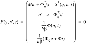
The SI2 Formulation
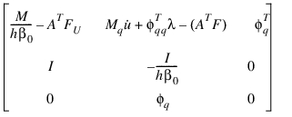
Gear, Gupta, and Leimkuhler have shown that drift-off can be prevented by appending Equation (33) to (31) and adding a new set of variable as follows:
 | (36) |
The numerical solution of Equations (36) are guaranteed to satisfy both  and
and  . In this sense, the Equations (36) are stabilized. Because the constraints
  have been differentiated once, Equation (36) has an Index = 2.
and . In this sense, the Equations (36) are stabilized. Because the constraints have been differentiated once, Equation (36) has an Index = 2.Equations (36) are called the Stabilized Index Two representation of Equations (31), (32), and (33). It has been proven that Equation (36) and Equation (31), (32), and (33) have the same solution when  = 0. This condition is rigorously enforced by the SI2 formulation in Adams Solver (C++).
= 0. This condition is rigorously enforced by the SI2 formulation in Adams Solver (C++).It can also be shown that the Jacobian of Equation (36) does not become ill-conditioned as h moves closer to 0. Furthermore, since Equation (36) has an Index of 2, the integrators can monitor integration error on both u and q.
Benefits and Limitations
The benefits and limitations of the SI2 formulation are described in the following table:
Characteristics of the SI2 Formulation
Benefits of the SI2 formulation: | Limitations of the SI2 formulation: |
|---|---|
■Gives very accurate results, especially for velocities and accelerations. ■Usually allows an ERROR that is approximately 10 to 100 times larger than regular GSTIFF to produce the same quality of results. ■Is very robust and stable at small step sizes. ■Corrector failures that small step sizes cause occur less frequently than with the Index-3 GSTIFF formulation. ■Singular matrices due to small step sizes occur less frequently than with the Index-3 GSTIFF formulation. ■Corrector failures are typically indicative of a modeling problem and not of a numerical deficiency in the Adams Solver software. ■Tracks high frequency oscillations very accurately. | ■Is typically 25% to 100% slower for most problems than regular GSTIFF, when run with the same error. ■Requires that all velocity inputs be differentiable. Therefore, you must define your MOTIONS so that they are smooth and twice differentiable. Non-smooth motions, which theoretically cause infinite accelerations, cause failures in the SI2 formulation. The I3 formulations can sometimes handle such models. |
WSTIFF
WSTIFF is a stiffly stable, BDF-based, variable-order, variable-step, multi-step integrator. It has a maximum order of six. The BDF coefficients it uses are a function of the integrator step size. Thus, when the step size changes in this integrator, the BDF coefficients change. WSTIFF can change step size without any loss of accuracy, which helps problems run more smoothly. The benefits and limitations of WSTIFF are the same as those of GSTIFF and are listed in the Characteristics of GSTIFF Integrator table.
References
For information on the WSTIFF integrator, see the paper:
■Van Bokhoven, W.M.G. (1975, February). Linear Implicit Differentiation Formulas of Variable Step and Order. IEEE Transactions on Circuits and Systems, 22 (2).
The HHT and Newmark Integrators
The HHT integrator is based on the  -method proposed by H.M. Hilber, T.J.R. Hughes, and R.L. Taylor [1]. The
  -method is widely used in the structural dynamics community for the numerical integration of second order ordinary differential equations that are obtained at the end of finite element discretization. If the finite element approach is linear, the equations assume the form:
-method proposed by H.M. Hilber, T.J.R. Hughes, and R.L. Taylor [1]. The -method is widely used in the structural dynamics community for the numerical integration of second order ordinary differential equations that are obtained at the end of finite element discretization. If the finite element approach is linear, the equations assume the form: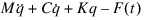 | (37) |
The mass, damping, and stiffness matrices, M, C, and K, respectively, are constant, and the force F depends on time.
The  -method comes from the Newmark method proposed by N.M. Newmark [3], which defines a family of integration formulas that depend on two parameters
  and
and  .
.
-method comes from the Newmark method proposed by N.M. Newmark [3], which defines a family of integration formulas that depend on two parameters and .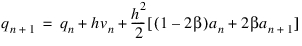 | (38) |
 | (39) |
In the Newmark formulation, these formulas are used to discretize the equations of motion (37)
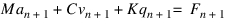 | (40) |
where an+1, vn+1, and qn+1 are numerical approximations for  ,
,  , and
, and  respectively.
, , and respectively.The Newmark method is implicit and A-stability (stability in the whole left plane) is guaranteed as soon as:
 | (41) |
 | (42) |
The Newmark method is an order one integration method, unless  and
and  , which makes the Newmark method same as the trapezoidal rule, which is a second-order method. The drawback of the trapezoidal rule is that it has poor damping properties, which is unacceptable for problems that have either:
and , which makes the Newmark method same as the trapezoidal rule, which is a second-order method. The drawback of the trapezoidal rule is that it has poor damping properties, which is unacceptable for problems that have either:■High oscillations that are of no interest
■Parasitic oscillations that are a byproduct of the finite element discretization process
The  -method came as an improvement as it preserved the A-stability of the Newmark formulas, while achieving second-order accuracy when used with the second-order linear ODE problem of Equation (37). The change to obtain this improvement does not pertain to the formulas proposed by Newmark, but rather the form of the discretized equations of motion in (40). The new equation in which the integration formulas of equations (38) and (39) are substituted is:
-method came as an improvement as it preserved the A-stability of the Newmark formulas, while achieving second-order accuracy when used with the second-order linear ODE problem of Equation (37). The change to obtain this improvement does not pertain to the formulas proposed by Newmark, but rather the form of the discretized equations of motion in (40). The new equation in which the integration formulas of equations (38) and (39) are substituted is: | (43) |
where
 | (44) |
The equations of motion associated with multi-body dynamics simulation in Adams are:
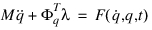 | (45) |
These equations are neither linear, nor ordinary differential as is the case in equation (37), because the solution q(t) must also satisfy the kinematic constraint equations:
 | (46) |
Looking at equation (43), the idea behind the HHT discretization is that the  -scaling is done in conjunction with the forces applied on the system. The current value of the force is first scaled by 1 +
  , while the value of the force at the previous time step is subtracted after being scaled by
  . According to equation (45), for the equations of motion in the multi-body formulation, the force is computed as
 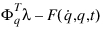 ; (that is, everything that is not explicitly depending on acceleration
  ). Therefore, in relation to the original HHT formulation, the discretization of the multi-body dynamics equations of motion is:
-scaling is done in conjunction with the forces applied on the system. The current value of the force is first scaled by 1 + , while the value of the force at the previous time step is subtracted after being scaled by . According to equation (45), for the equations of motion in the multi-body formulation, the force is computed as ; (that is, everything that is not explicitly depending on acceleration ). Therefore, in relation to the original HHT formulation, the discretization of the multi-body dynamics equations of motion is: | (47) |
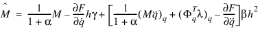
From an implementation standpoint it is more advantageous to scale the equation above by (1 +  ) and obtain the equivalent form:
) and obtain the equivalent form: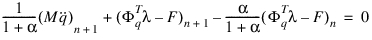 | (48) |
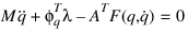
The second set of equations that must be satisfied at time tn+1 are the position kinematic constraint equations:
 | (49) |
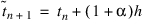
Using the notation:

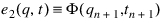
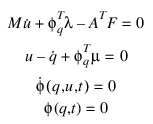
the simulation is advanced from time tn to tn+1, by finding the solution of the nonlinear system:
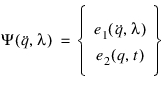 | (50) |
The unknowns solved for are  and
and  . Note that although q and
  appear in equation (50), they are expressed in terms of
  based on the formulas of equations (38) and (39) (the notation used there was v for
  , and a for
  ). These integration formulas define linear relationships of the form
 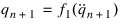 and
and 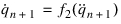 . It is easy to see that based on equations (38) and (39)
and . Note that although q and appear in equation (50), they are expressed in terms of based on the formulas of equations (38) and (39) (the notation used there was v for , and a for ). These integration formulas define linear relationships of the form and . It is easy to see that based on equations (38) and (39)
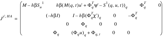
The Jacobian of the nonlinear system of equation (50) is given by:
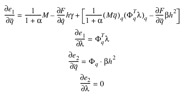
Using the notation:
 | (51) |
one correction in the quasi-Newton algorithm is computed as the solution of the linear system:
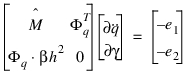 | (52) |
To balance the coefficient matrix in the previous linear system, the last row is scaled by  :
:
: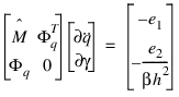 | (53) |
The correction at iteration k is then applied as:
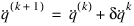 | (54) |
 | (55) |
and the corresponding  and
and  are computed using the new value
  and equations (41) and (42), respectively.
and are computed using the new value and equations (41) and (42), respectively.The role of the corrector is to calculate the quantities  and
and  at the new time step tn+1. After these quantities are computed the accuracy of the results at the current step is verified against the user-specified error tolerance. If the local integration error is less than the user-specified error the integration step is accepted; otherwise, it is rejected and a new smaller step size is tried.
and at the new time step tn+1. After these quantities are computed the accuracy of the results at the current step is verified against the user-specified error tolerance. If the local integration error is less than the user-specified error the integration step is accepted; otherwise, it is rejected and a new smaller step size is tried.For more information on error-estimation step-size selection and corrector-stopping criteria, refer to Simcompanion Knowledge Base Article KB8016154
Remarks:
■The following explains how the HHT and Newmark integrators are more efficient than the default GSTIFF integrator:
1. The most time-consuming part of simulation is the computation of the Jacobian associated with the nonlinear discretization system. The HHT integrator contains heuristics to reduce the number of Jacobian evaluations as much as possible. Unlike the BDF integrator, where terms of the integration Jacobian can become disproportionately large as a result of a scaling by the inverse of the step-size, the HHT integrator employs a different approach, where certain values are multiplied (never divided) by the step-size before populating the Jacobian. As long as the step-size does not change dramatically, this approach better supports the recycling of the Jacobian over several consecutive time-steps.
2. When compared with the BDF-based approach, the resulting HHT Jacobian is numerically better conditioned, which leads to more reliable corrections in the Newton-like iterative approach for large problems. Typically, at each integration step, this results in a smaller number of corrector iterations. In addition, because certain partial derivatives are scaled by the step-size, or the square of the step-size before populating the Jacobian, small errors in the partial derivatives computation will have a lesser negative effect on the overall quality of the Jacobian.
3. The BDF formulas of order higher than 1 contain regions of instability in the left plane. The higher the order, the smaller the region of stability. In addition, BDF is intrinsically designed to maximize the order and step-size of the integration. Because of these two conflicting attributes, particularly for models that are mechanically stiff (models with stiff springs, flexible bodies), there are many instances when a order/step-size choice puts the BDF integrator outside the stability region. These integration time-steps are typically rejected, and smaller step-sizes are required to advance the simulation. This is not an issue with the HHT integrator, which is a fixed low order method (second order for HHT, mostly first order for Newmark).
4. The HHT is a one-step integration formula that further gives it a small edge over multi-step methods, such as high-order BDF-type integrators.
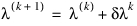
■In the HHT, the  coefficient can assume any value in the range -0.3 <
  < 0. Once a value is selected, the
  and
and  coefficients of equations (38) and (39) are computed as:
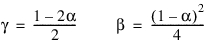
coefficient can assume any value in the range -0.3 < < 0. Once a value is selected, the and coefficients of equations (38) and (39) are computed as:■The Newmark method effectively sets  = 0 and then you are responsible for defining values for
  and
and  that satisfy equations (41) and (42). Typical values are
  = 0.7 and
  = 0.36.
= 0 and then you are responsible for defining values for and that satisfy equations (41) and (42). Typical values are = 0.7 and = 0.36.■The priority of the HHT and Newmark integrator is speed rather than accuracy. If accuracy is of concern, the current integrators available in Adams historically are very accurate and serve the purpose well.
■The HHT and Newmark error control for DIFF, TFSISO, LSE, and GSE elements is significantly more lax than the one carried out for these elements by the other integrators available in Adams Solver (C++) (such as GSTIFF, WSTIFF, and so on). This is related to the nature of the HHT and Newmark integration formulas, which deal exclusively with second-order differential equations. To have these formulas accommodate DIFF's for example, these are first converted from first- into second-order differential equations. The consequence of this transformation is that error control is now performed on the integrals of the DIFF states, rather than on the actual states. As far as smoothness is concerned, it is well known that an integral of a quantity is better behaved than the quantity itself. Consequently, the HHT and Newmark integrators are typically more optimistic in selecting integration step-sizes. While these step-sizes are fine for the level or error induced in the integral of the DIFF's, sometimes they are too aggressive, which negatively reflects to the quality of the actual states associated with the DIFF's. HHT and Newmark in the current implementation are not recommended for models whose time evolution (or behavior) is dominated by elements, such as DIFF, TFSISO, LSE, or GSE.
■The default ERROR for HHT and Newmark is 1.E-5. This tighter default value is intended to counterbalance the different step-size selection strategy employed by these integrators, and can be regarded as a calibration procedure. The goal is that working with the corresponding default values of the ERROR attribute both the HHT and GSTIFF integrators will produce results of similar quality.
Note that the default integrator in Adams Solver (C++) is GSTIFF, and, therefore, the default ERROR associated with a simulation is 1.E-3. GSTIFF and ERROR=1.E-3 are the settings that are provided to the solver if in the .adm file you do not explicitly sets these attributes through the INTEGRATOR statement.It is important to understand that under these circumstances, if you later change the integrator to HHT through a command issued in the .acf file, unless the command explicitly specifies otherwise, the ERROR value of 1.E-3 (associated with GSTIFF) will be inherited. The correct command to issue would be INTEGRATOR/HHT, DEFAULT, if the goal were to run HHT with its default ERROR setting, that is ERROR=1.E-5. Learn more in the INTEGRATOR command.
Benefits of the HHT and Newmark Integrators | Limitations of the HHT and Newmark Integrators |
|---|---|
■Expected to result in a smaller number of Jacobian evaluations. ■Unlike BDF-type formulas, behaves like a low pass filter; it cuts high frequency spurious oscillations, while accurately preserving low frequency oscillations. ■Can control the cutoff frequency by adjusting  ; the smaller value (that is, closer to -0.3, the lower the cutoff threshold). ; the smaller value (that is, closer to -0.3, the lower the cutoff threshold).■Stable at small value of the integration step size. | ■Because of the reduced order, the acceleration and reaction forces obtained with this I3 formulation are going to be more spiky. ■The numerical damping associated with HHT is smaller than the one produced by BDF integrators used by the GSTIFF family. ■If a BDF-based integrator manages to run a simulation at order 4 or higher, it will take step sizes significantly larger than HHT. This is because HHT is a low-order integrator and it needs to limit the step size based on accuracy characteristics. |
References
1. H. M. Hilber, T. J. R. Hughes, and R .L. Taylor. Improved numerical dissipation for time integration algorithms in structural dynamics. Earthquake Eng. and Struct. Dynamics, 5:283292, 1977.
2. D. Negrut. On the implementation of HHT and Newmark integrators in MSC.ADAMS. Knowledge Base Article KB8016154.
3. N. M. Newmark. A method of computation for structural dynamics. Journal of the Engineering Mechanics Division, ASCE, pages 6794, 1959.
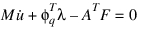
HASTIFF
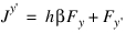
solving for y’ (y discretized as a function of y’):
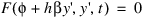
HASTIFF is the integrator in Adams Solver (C++). It is a variable-order, variable-step, multi-step integrator with a maximum integration order of six. The BDF coefficients it uses are calculated by assuming that the step size of the model is mostly constant.
Characteristics of HASTIFF(Hiller - Anantharaman ) integrator
1. Lagrange Multipliers appear in their differential form .
2. Solving for y ', instead of y (y is discretized as a function of y')
3. The constrained are scale by 1/h1. (h=steps-size,
  is the BDF coefficient that multiplies y’).
(h=steps-size, is the BDF coefficient that multiplies y’). 4. The formulation is Stabilized Index-1: an index-1 formulation is preferable because it’s more stable numerically, hence it potentially allows for bigger and fewer steps to reach the end-time.
5. Stabilized Index-1 (SI1) and Stabilized Index-2 (SI2) are available for HASTIFF. SI1 is the default for HASTIFF.
The I1(Hiller - Anantharaman index -1 ) Formulation
Characterstics of index -1 formulation.
1. Ensures that the solution satisfies all both position and velocity constraints.
2. Does ensure that the velocities and accelerations calculated satisfy all first- and second-time derivatives.
3. Monitors integration error only in system displacements and velocities.
4. Is as fast as GSTIFF SI-2.
5. The Jacobian matrix *cannot* become ill-conditioned even at small step sizes
See the theory of HASTIFF
Error in Handling Simulations
The following sections include descriptions and workarounds for common error conditions you might encounter during a simulation. The sections include:
Integration Failures
An integration failure is the condition when the integrator calculates a solution, but then rejects it because it does not meet the accuracy requirements you specified. Because all integrators attempt to take the largest time step possible, failure is a fairly routine occurrence and is not cause for concern. Integrators can automatically decrease the step size and/or integrator order and repeat the step. Integration failures in multi-step methods are caused when the predictor and corrector lead to vastly different configurations. Such a situation can occur often when a force is suddenly turned on or off, thus, causing a discontinuity in the solution. For this reason, past values are not a good indicator of current values. The following tips can help you avoid integration failure:
■When modeling, be sure that all motion inputs, user-defined forces, and user-written differential equations are both continuous and differentiable. The smoother a function is, the easier it is to integrate. Always use a STEP or, better yet, the STEP5 function to switch a signal on or off, instead of using IF logic.
■Remember that cubic SPLINEs can only guarantee second-order differentiability. Inputting a SPLINE through a displacement-based MOTION causes accelerations to be spiky. Therefore, input the SPLINE in a velocity-based MOTION.
■For greater simulation control, use HMAX to control the maximum step size that the integrator can take. HMAX enables the integrator to reach higher orders and maintain them consistently.
■Be careful when using non-differentiable intrinsic functions, such as IF, MIN, MAX, SIGN, MOD, and DIM. These functions can give discontinuous answers and can cause integrator problems. The integration failure diagnostic identifies the variable and its parent modeling element with the largest error. Examine the entities that connect to the parent modeling element to see if you can identify the cause of the failure.
Corrector Failures
A corrector failure occurs when the Newton-Raphson iterations in the correction phase do not converge to a solution. Corrector failure occurs if the predictor cannot provide a reasonable initial guess and the equations themselves are not smooth, as the Newton-Raphson algorithm assumes. A corrector failure is a fairly severe event that you should avoid by changing your model. Some tips to help avoid corrector failure are:
■As with preventing integrator failures, be sure that all motion inputs, user-defined forces, user-written differential equations, and user-defined algebraic variables are both continuous and differentiable. The smoother a function is, the easier it is to solve for it. Use a STEP or STEP5 function to switch a signal on or off instead of using IF logic.
■Use the ERROR keyword to loosen the integration error. Loosening the value for ERROR also decreases the tolerance that the corrector is required to meet.
■Use the SI2 formulation and see if the failures go away.
■Use the new corrector by setting CORRECTOR = MODIFIED.
Here are some diagnostic techniques for identifying the cause of some failures:
■Examine the EPRINT output from DEBUG to identify the modeling entities that are having the greatest difficulty converging.
■If the modeling element is a force:
■Make sure that the force law it obeys is smooth.
■Examine the stiffness of the force entity. Reduce it if necessary to overcome the failures.
■Examine the damping of the force entity. Damping is usually less than 5% of the stiffness. Large values of damping can also cause failures.
■If the modeling element causing the corrector failures is an equation of force/torque balance for a PART, POINT_MASS, or FLEX_BODY, try to identify the entities that may be applying anomalous forces on the body. Look at the accelerations of the body. A large acceleration in a certain direction is always caused by a large force in that direction. Try to identify the modeling element that is causing the large acceleration, examine how it is defined, and try to understand why it is applying a large force.
■If the modeling element is a CONTACT, review the stiffness, damping, and frictional properties of the contact. Reducing stiffness and damping helps. Similarly, increasing stiction and dynamic friction transition velocities can help the integrator.
■If the modeling element is a FRICTION entity, increasing the stiction and dynamic friction transition velocities usually helps. Evaluate the effect of reducing the friction coefficients and the pre-load.
■If the modeling element is a DIFF or GSE, make sure that the derivatives you are defining have reasonable values. Large derivatives cause problems. Make sure that the constitutive equations are smooth (differentiable) and that they do not have any kinks.
■If the modeling element is a redundant constraint, this implies that Adams Solver is having difficulty satisfying the constraint. The most likely cause for such a failure is an inconsistently defined or ill-behaved model. Eliminate the inconsistency.
■If the modeling element is a constraint reaction, try to identify the applied force or torque that is trying to break the constraint.
Integration Restarts
An integration restart is when the integrator fails to take a new step successfully. Adams Solver (C++) calculates a new and consistent set of initial conditions at the point of failure and the solution progresses with this new set of initial conditions. A restart occurs if the integrator encounters several consecutive integration failures and/or corrector failures while attempting a new step. Integration restart is usually indicative of discontinuous equations describing the system. To help avoid integration restart, you can:
■Increase ERROR value. Integration restarts sometimes occur simply because the value specified for ERROR is too small.
■Identify modeling problems in your system. Typically, a single modeling element dominates an integrator or corrector error. Identify that element and see why it may be causing problems. Smoothen its definition if there is a function expression or user subroutine associated with it. For more information on how to diagnose modeling problems, see Corrector Failures.
Singular Matrices and Symbolic Refactorization
A singular matrix condition occurs when the Jacobian matrix is not invertible. Recall that the corrector needs to invert the Jacobian matrix during its iterations to solve a set of linearized algebraic equations. (See Correction). A scalar analogy to a singular matrix is a divide-by-zero situation. Adams Solver (C++) does not actually invert the matrix, but calculates the matrixs Lower and Upper triangular factors (LU factors). This method of computation is very efficient and is equivalent to an inversion.
Given a Jacobian matrix, Adams Solver (C++) calculates and stores the LU factors in a symbolic form. In other words, Adams Solver (C++) explicitly calculates the LU factors as a function of the values in the Jacobian matrix. Adams Solver (C++) also assumes that the pivots are never zero. (Pivots are chosen during the Gaussian elimination and are used to factorize the matrix.) Because the equations being solved are nonlinear, it is likely that a set of pivots chosen earlier may not be optimal. Some of the pivots may become small or even zero. This event is known as the singular matrix condition. When Adams Solver (C++) encounters this condition, it recalculates the symbolic LU factors for the Jacobian matrix using the current values of the state variables. This process is known as symbolic refactorization.
Occasional occurrences with singular matrices and symbolic refactorization are normal and are no cause for alarm. However, if these events occur frequently, you should examine your model. The typical causes for singular matrices are:
■A mass or inertia component is not specified.
■The system has reached a locked configuration, that is, it can no longer move without violating one of its constraints.
■A large force or moment has been suddenly turned on or off.
■The integrator is forced to take an extremely small step because of a hidden discontinuity in an element described in a user-written subroutine. IF statements, as well as non-differentiable intrinsic functions, such as SIGN, MOD, MIN, MAX, and so on, can create non-differentiable or even discontinuous descriptions of modeling elements. Be very careful when using these aspects of a programming language.
The Index-3 Jacobian matrix (see Equation 6) contains some terms that are inversely proportional to the step size being taken. As the step size shrinks, these terms grow larger. In fact, they grow so large that they eclipse all other entries in the matrix. Computers typically have difficulty dealing with matrices that have entries spanning a large range (matrices with large condition numbers). The smaller numbers consequently get lost in round-off error, and, therefore, cause singular or ill-conditioned matrices to occur. The root cause for these problems is that the step size is very small. The solution is to understand why the step size is so small, and modify the model accordingly. Discontinuities are prime causes for problems related to small steps sizes. Eliminating the discontinuities causes the integrator to take larger steps, and, therefore, avoid fatal singular matrix condition. Using the SI2 formulation can also help solve this problem.
Choosing and Integration Error
The integration ERROR is a key parameter that you need to specify for a simulation. For calculating a reasonable value for ERROR, we recommend that:
■For I3 formulation with GSTIFF and WSTIFF:
ERROR = VEPS *(6*Nb + 3*Np + Nu + 2*Nm)
■For SI2 formulation with GSTIFF and WSTIFF:
ERROR= K * VEPS * (12*Nb + 6*Np + Nu + 2*Nm)
where:
VEPS is the desired error per variable per integration step.
Nb is the number of rigid bodies in the model (excluding GROUND).
Np is the number of point masses in the system.
Nu is the number of user-defined differential equations in the system (DIFFs+LSEs+GSEs).
Nm is the total number of modal coordinates in the system:
■K =10 (for smooth problems).
■K =100 (for impact and friction problems).
■For HHT and Newmark integrators, use the error that you would use for GSTIFF but typically scaled by a factor of 10-2.
All integrators require that you input a value, referred to as ERROR in the online help, that specifies the degree of accuracy you want to achieve in a simulation. ERROR is the maximum error allowed per integration step for the entire system. This can be confusing in Adams Solver (C++) because some of the ERROR states are displacements, some are velocities, and others may be user-defined states (for example, pressure, and temperature).
In Adams Solver (C++), integration ERROR is the difference between the exact solution f(t) and the approximate solution p(t) being calculated. The difference, f(t)-p(t), is the truncation error.
For displacement variables, the truncation error has units of length. For velocities, the truncation error has units of velocities. For example, if you are working in millimeters, your maximum error tolerance would be smaller than 1 micron. Then, for each variable, you would have an error of 0.001 mm.
You find the error per step by estimating the total number of integration steps, and then dividing the error per variable by the estimated number. Thus, if you estimate that you need 100 integration steps, the error per step, VEPS, is 0.00001 mm. This is always a conservative calculation (sometimes too conservative) because errors tend to be random and typically cancel each other out. The calculation shown earlier assumes the worst case scenario, where the errors are always additive. You should use the information shown here as a guide, not as a rule, for setting ERROR.
Velocities must be treated in the same way as displacements. However, keep in mind that the errors in the derivatives are higher, and, if you impose an error on the velocities that are identical to the errors on the displacements, you force a larger number of iterations per step to occur, which increases the simulation time. In general, if an error-control exists on velocities, such as in SI2 and ABAM, then the errors computed for the displacements can be increased by a factor of 10 and can also be applied for velocities.
Modal coordinates have small values, and, therefore, to be able to accurately capture their effects, you may need to tighten the ERROR parameter. Typically, when the rigid body displacements and velocities are accurate, then the modal coordinates and velocities are also fairly accurate.
Models with Discrete GSEs
Each integrator has a proprietary algorithm to select the next time step. Each algorithm selects the next time step taking into consideration parameters set by the user (for example, HMAX), the proximity to an output time step, integration error and so on. However, when a model has discrete GSE elements in it, the integrator first computes a proposed time step and then reviews the sample periods of all discrete GSEs in the model. If the proposed time step would set the system at a new time beyond a scheduled sample period, then the time step is reduced so the system does not step beyond a sample period. In a case of the constant sample period, the output step size (DTOUT) should be selected as an integer multiple of the sample period of the discrete GSEs in the model for optimal solver performance.
Fixed Step Integrator Option
The fixed step option is introduced for the GSTIFF integrator supporting both the I3 and SI2 formulations and for the HHT integrator. The purpose of the fixed step option is to ensure that a fixed amount of work is completed in a given time to satisfy the requirements for a Linux real time operating system (RTOS). This is achieved by limiting the number of Newton steps in the implicit solve (that is, number of corrector iterations per integration time-step) to ensure a fixed amount of work is performed.
This option can be employed regardless of the environment; that is, it can be used also in non-RTOS scenario, for example, to help determine ahead of time if a given analysis can be suitable for real-time simulation and if the results will be acceptable. The fixed step option will be employed 'only' when the user specifies FIXIT. It should be noted that the integration step size remains 'constant' or 'fixed' throughout the simulation when the fixed step option is selected. The combination of DTOUT and HRATIO settings specifies the integration step size as shown in the following figure:
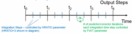
■The dependencies of the other INTEGRATOR statement/command arguments when FIXIT is specified are as follows:
■MAXIT will be ignored
■ERROR will be ignored
■INTERPOLATE will be ignored and always treated as though it is set "OFF"
■HINIT can still be specified, but if set >DTOUT/HRATIO then Adams Solver will reset it = DTOUT/HRATIO
■HMIN will be ignored
■HMAX can still be specified but will be ignored if less than DTOUT/HRATIO
■KMAX can still be specified but will have no effect since the fixed step GSTIFF always runs with K=1 and HHT always runs with K=2. So, in effect we have a fixed step and fixed order integrator
■CORRECTOR type will have no effect
■PATTERN can still be specified; note that default for GSTIFF remains T:F:F:F:T:F:F:F:T:F. This is suitable for values of FIXIT less than or equal to 4. If larger values of FIXIT are necessary one may want to consider setting PATTERN = T:F:F:F:F:F:F:F:F:F so as to avoid the time consuming Jacobian re-evaluation during newton iterations for real-time performance. Adapative Jacobian evaluation (that is, PATTERN = F) is not supported in the fixed step integrator as it does not guarantee the fixed amount of work per time step. Note that the default pattern for HHT is changed to T:F:F:F:T:F:F:F:T:F when the fixed step option is selected.
Suggested modeling practices with the fixed step integrator:
Discontinuities in Adams Solver, especially in the 0th and 1st derivatives, whether from function expressions or from user-written subroutines, etc. are common source of solution failures even using the traditional variable step integrators. Problems with discontinuities will likely be exacerbated when using the fixed step integrator. Below is a list of suggested modeling practices in this regard:
■Do not use non-holonomic constraints
■Manually remove/resolve redundant constraints as opposed to letting Adams Solver automatically remove these
■Scrutinize any IF statements in function expressions and, if they cause discontinuities, replace them with STEP functions
■Consider analytic type alternatives to any surface-surface contacts
■Check the damping specifications in CONTACT and IMPACT elements against units. Strongly consider avoiding damping penetration distances that are <0.001 length unit and damping values that are >.01 * stiffness values.
■Avoid velocities which oscillate around zero. This can be common in certain kinds of friction scenarios as well as bringing vehicle models to a stop
Handling sensors, contacts and discrete GSEs with the fixed step integrator:
The fixed step integrator supports the contact, sensors and the discrete GSEs. However, it does not honor any step size change requests coming from these elements. The user should choose the constant step size (using DTOUT and HRATIO combination) carefully when the model contains one of these elements. The discrete GSE states will be updated every time step. For example, when Adams Smart Driver is used it is the user's responsibility to select the 'fixed' step size such that it will be smaller than (or equal to) the discrete GSE (in this case, 'SamplePeriod' in the driver control file).
Amplification of initial transients with the fixed step integrator:
Users should take extra care with models exhibiting initial transients in their results from the traditional variable step integrators. If the model/event is not corrected to eliminate such initial transients they may very likely be amplified when running the model with the fixed step integrator. Even relatively small amplitude initial transients in the variable step integrator which a user might not deem important enough to worry about normally can become amplified and problematic in the fixed step integrator.
Integrator restarts with the fixed step integrator:
It should be noted that the fixed step integrator option does not support 'integrator restarts.' This is done intentionally to avoid the extra amount of computation associated with integrator restarts and also to guarantee the fixed amount of work per integration time step. Integrator restarts are generally caused by i. Singular or ill-conditioned Jacobian, ii. Discontinuity in forces, iii. Sensors forcing the integrator restart, or iv. Euler Singularity. Ideally the user should avoid all these conditions when the fixed step integrator option is selected. Note that the Euler singularity case is supported in the fixed step integrator option without forcing an integrator restart.
Running with the fixed step integrator in real-time environments
If running Adams as an FMU in real-time environments, see options for the FMU parameter msc_adams_realtime in section Default fixed parameters in an Adams FMU, and the documentation for the environment variable MSC_ADAMS_REAL_TIME. The FMU parameters and the environment variable provide options for controlling the generation of output results, messages, and other integrator parameter settings.
Real Time Index (RTI) reporting with the fixed step integrator:
When using a fixed step integrator in real-time environments, Adams Solver (C++) will print (in both the message file and the display) a report about the Real Time Index (RTI) measured during the dynamic simulations. The Real Time Index is defined as the ratio t_elapsed to t_step where,
t_elapsed = wall time required by Adams Solver (C++) to step the system a single time step.
t_step = time step requested by the controller code (or set by the DOUT/HRATIO options).
A value for the RTI less than 1.0 means Adams Solver (C++) was able to step the system fast enough in a real time environment. The printed report includes a heading with the following information:
a. The name of the fixed step integrator being used.
b. The time units of the model.
c. The HRATIO used in the INTEGRATOR statement or command.
d. The size of the time step requested in both user's units and in seconds.
e. The requested frequency in Hz.
The report also includes:
a. The value of the minimum measured RTI during the simulation. The reported value includes the corresponding frequency and the simulation time when this minimum value was measured.
b. The value of the average measured RTI for all the simulation and corresponding frequency.
c. The value of the largest measured RTI during the simulation. The reported value includes the corresponding frequency and the time when this largest value was measured.
By default, the RTI report excludes the value of the first-step RTI. The first-step RTI is typically larger than all subsequent RTIs because it has the overhead of data initializations. This behavior is standard in all real time systems but it is of no concern given that real time simulations usually begin with trivial maneuvers before the actual simulation of interest begins.
An example output is as follows:
--------------------------------
Real Time Index (RTI) statistics
--------------------------------
Integrator name : Fixed Step GSTIFF/I3
Time units : s (seconds)
HRATIO : 2
Time step : 5.00000e-02 s
Requested frequency : 100.00 Hz
Minimum RTI index : 0.29999 (333 Hz) (at time 2.000000e-02 s)
Average RTI index : 0.38838 (257 Hz)
Maximum RTI index : 0.60001 (166 Hz) (at time 3.000000e-02 s)
Notes:
1. Minimum, Average and Maximum RTI are computed after the first integration step.
2. The frequency (Hz) is measured as the inverse of the time (seconds) required to step one whole step.
3. A zero RTI was detected. This is a limitation of the OS granularity in measuring CPU time.
Notes: | Setting the environment variable MSC_ADAMS_SOLVER_INTERPOLATE_ADAPTIVE enforces Adams Solver to use a different output block generation. The scheme works as follows: ■Instead of generating an output block at each requested interval provided in the SIMULATE/DYNAMICS command, Adams Solver ignores the request of generating equally spaced output blocks and generates an output block at any integration step past the request interval. The end result is that Adams Solver generates output blocks at unequally spaced times. ■Using this setting, the solver does not need to reduce the current time step in order to hit a requested output block. Instead, it leaps over and prints an output block as soon as a request output block was suggested. In some cases, the solver may leap over more than one requested output blocks. The main benefit is speed performance. The main drawback is that output blocks are not equally spaced. |
Tip: | GSTIFF and WSTIFF control errors specifically in displacements and user-defined differential variables, and, therefore, yield acceptable accuracy in velocity, acceleration, and force results. In some cases, however, the acceleration and force results may not be acceptable, even when ERROR is set appropriately and the displacement results are accurate. In these cases, use the HMAX argument to directly limit the size of the integration steps. Using the PATTERN argument to request more frequent evaluations of the Jacobian matrix can improve convergence rates. This can also increase the computation time. For kinematic (zero-DOF) systems, a kinematic analysis is usually faster and less expensive than a dynamic analysis. To force the integration of a kinematic system, use GSTIFF, WSTIFF, HHT, or Newmark. |
Caution: | GSTIFF, HHT, and Newmark may introduce discontinuities in velocities and accelerations when the integration step size changes. Most of the time, these discontinuities are within the error tolerance and disappear quickly. The use of the INTERPOLATE argument can sometimes eliminate these discontinuities. Alternatively, you can control the step size using the HMAX argument, which helps make the step sizes nearly constant. The HHT integrator is incompatible with restitution (POISSON) contact. |
Examples
■INTEGRATOR/SI2, GSTIFF, ERROR=1.0E-4, HINIT=1.0E-6
This integrator statement specifies that dynamic simulations be run using the SI2 equation formulation combined with the GSTIFF integrator.
♦This solution has an error limit of 1.0E-4.
♦The integrator is to take an initial step of 1.0E-6.
■INTEGRATOR/HHT, ERROR=5.0E-6, PATTERN=F, HMAX=1e-3
This integrator statement specifies that dynamic simulations be run using the HHT integrator with the adaptive jacobian pattern.
♦This solution has an error limit of 5.0E-6.
♦The maximum step size the integrator is to take is 1.0E-3.
■INTEGRATOR/GSTIFF, I3, FIXIT =3, HRATIO = 4, MAXERR = 0.5
This integrator statement specifies that dynamic simulations be run using the fixed step integrator (GSTIFF-I3) option.
♦The number of corrector iterations per time step is 3 throughout the simulation.
♦The ratio of DTOUT (output step size) to H (integration step size) is 4 throughout the simulation.
♦The simulation will be stopped if the integration local error exceeds 0.5
See other Analysis parameters available.