Isolator-Parameter Identification Tool with Aview (IPIT)
The Isolator-Parameter Identification Tool (IPIT) has been developed to identify the parameters of the non linear frequency and amplitude dependent bushing models in Adams out of bushing measuring data in terms of dynamic stiffness and damping. The output of the identification process is a bushing property file that contains all the parameters for the bushing so it can be used in your model.
The IPIT can deal with two types of bushing models:
1. The general bushing model (files with .gbu extension), a 6 DOF model using a combination of transfer functions, the Bouc-Wen model and a static spline, see 'How to use IPIT for the general bushing parameters'.
2. The hydromount model (files with .hbu extension), a one dimensional model that can represent amplitude and frequency dependent characteristics as shown by hydromounts, see 'How to use the IPIT for the hydromount bushing parameters'.
Note: | This model is not currently available through the Adams View interface. |
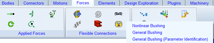
For starting the IPIT click on Ribbon → Forces → Flexible Connections → General Bushing (Parameter Identification)
How to use IPIT for the general bushing parameters
Learn more about the IPIT for general bushings:
IPIT GUI for General Bushing file optimization
Click on Ribbon → Forces → Flexible Connections → General Bushing (Parameter Identification). This will open the IPIT GUI and then click on File → Load File and select the bushing property 'gen_bus003.gbu' from the <top_dir>/aview/examples/bushings:
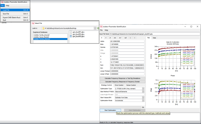
The IPIT is able to determine parameters for each direction of the gbu for which data has been provided in one of the BUSHING_TEST_DATA blocks:
BUSHING_TEST_DATA_X
BUSHING_TEST_DATA_Y
BUSHING_TEST_DATA_Z
BUSHING_TEST_DATA_AX
BUSHING_TEST_DATA_AY
BUSHING_TEST_DATA_AZ
The sections with BUSHING_IDENT I E'ICAT ION_DATA are generated by the IPIT and represent the calculated response of the bushing model for the test data points.
With the top toolbar the user can Load or Save a .gbu bushing property file. Additionally, there is quick access to the online help for IPIT and finally the option to Export the bushing CMD file. This option can be used to run the IPIT in batch mode with Adams. For more information about running the IPIT, please refer the section Running IPIT in Batch Mode.
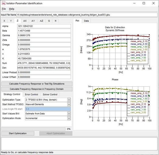
The GUI exists of 3 main panels, the first at the top left contains all the bushing parameters, organized in a tab for each direction. The tab will be set to the first direction for which data is available in the bushing property file, direction 'H' is used for the hydromount bushing. The IPIT will visualize and calculate the parameters for just this direction.
The X- to AZ-directions allows the user to fit the parameters for the general bushing using the 'Bouc-Wen hysteresis model as described below. The 'G'- direction provides the IPIT fitting capabilities for a user supplied model defined in a template file.
The bottom left section of the GUI contains all the governing parameters and settings for the identification process. On the right side there is the plot field, which displays the frequency response of the model; the dynamic stiffness in the plot is named Cdyn and the loss angle in the plot is named Phase. Finally, there is a second tab, the Data, which displays the input file and the tabulated frequency response data. At the bottom of the GUI, there is the progress bar and below that there is the status bar which lists some useful information about current status of the IPIT such as the objective function during the identification process.
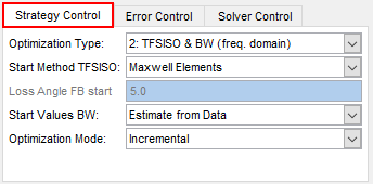
The figure below illustrates the three tabs which contains all the governing parameters referring to the identification process:
1. Strategy Control
Option | Definition and default value |
|---|---|
Optimization Type | 1. TFSISO (freq. domain) The optimization tool will calculate the parameters of the transferfunction (TFSISO), for BUSHING_COUPLING = 3 only. 2. TFSISO & BW (freq. domain) The optimization tool will calculate the parameters of the transferfunction (TFSISO) and the Bouc-Wen function (BW) in frequency domain, for BUSHING_COUPLING = 3 only. 3. TFSISO & BW (time domain) The optimization tool will calculate the parameters of the transferfunction (TFSISO) and the Bouc-Wen function (BW) in time domain using bushing test rig simulations (time domain). |
Start Method TFSISO | ■MaxWell Elements A set of parallel Maxwell Elements will be used to approximate the TFSISO parameters, applied in Optimization Type 1, for BUSHING_COUPLING = 3 only. ■Frequency Bushing A frequency Bushing approximation will be used to approximate the TFSISO parameters, applied in Optimization Type 1, for BUSHING_COUPLING = 3 only. |
Loss Angle FB start | Specifies the loss angle for the Frequency Bushing start method (in degrees). |
Start Values BW | ■Estimate from Data Start values for the Bouc-Wen function for Optimization Type 2 will be estimated from the Bushing Data, for BUSHING_COUPLING = 3 only. ■Actual Values The Bouc-Wen values as specified in the GUI will be taken Optimization Type 2, for BUSHING_COUPLING = 3 only |
Optimization Mode | ■Incremental The specified Optimization Type and its predecessors will be performed, for BUSHING_COUPLING = 3 only. ■Single Just the selected Optimization Type will be performed |
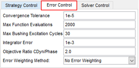
2. Error Control
Option | Definition and default value |
|---|---|
Convergence Tolerance | Supplying the tolerance constraint for which the objective function is considered to converge. Default:1e-5 |
Max Function Evaluations | Supplying the maximum function evaluation step allowed to be performed by the optimizer. Default: 2000 |
Max Bushing Excitation Cycles | The maximum number of cycles that the component testrig should use to derive the dynamic stiffness and loss angle in the bushing testrig simulations (Optimization Type 3) Default: 30 |
Integrator Error | Specifies the Adams Solver integration error used in the bushing testrig simulations (Optimization Type 3) Default: 1*10-3 |
Objective Ratio Cdyn/Phase | Specifies the objective ratio between Dynamic Stiffness and Loss Angle to be used in the objective error calculation by the optimizer, see below. Default: 2.0. |
Error Weighting Method (BUSHING_COUPLING = 2 or 3) | ■Weighting factor to be applied by the optimizer for the objective error function: Default one, no weighting ■1 / amplitude, the accuracy for points smaller at amplitudes will increase ■1 / sqrt(amplitude), the accuracy for smaller amplitudes will increase, but less pronounced as with 1/amplitude ■1/ sqrt(frequency), the accuracy for lower frequencies will be more pronounced ■1/ sqrt(amplitude*frequency), both smaller amplitudes and frequencies will be more accurate. |
The IPIT optimizer calculates the general bushing parameters by changing the bushing parameters aiming at a minimal difference in between the bushing data points and the bushing model response.
So actually the objective error function for the optimizer is:
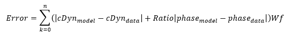
In which:
■cDyn is dynamic stiffness
■phase is the phase loss
■Ratio is the 'Objective Ratio CDyn/Phase'
■Wf is the weighting factor, by which one can influence the accuracy of the fit over the range of amplitude and frequency (BUSHING_COUPLING = 3 only).
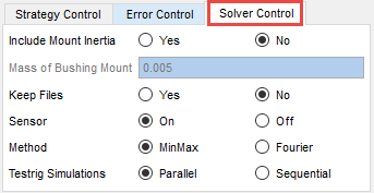
3. Solver Control
Option | Definition and default value |
|---|---|
Include Mount Inertia | Sets the optimizer method for accounting for the inertia effects of the bushing mounts in the bushing test rig simulations (Optimization Type 3) Default: No. |
Mass of Bushing Mount | When the Mount Inertia is included, the mass of the mount can be specified here. This mount part matches with the ‘ges_i_part’ in the Adams Ride assembly mdids://aride_shared/assemblies.tbl/component_general_bushing_example.asy for the component testrig. When comparing the results in the IPIT with the component testrig, this mass should be identical. |
Keep Files | The Adams Solver related files for the bushing test rig simulation (Optimization Type 3) are not deleted when set to Yes. This can be useful in case the test rig simulations are slow or not responsive or need debugging. Default: No |
Sensor | Activates or deactivates the Energy Sensor. When the sensor is activated the frequency response is captured during the time simulations of the bushing model (Optimization Type 3) and the simulation is terminated as soon the model has a stable response. Default: Activated |
Method | Selects the method to calculate the frequency response (dynamic stiffness and loss angle) during Optimization Type 3. Default: MinMax |
Testrig Simulations | Chooses to run the Adams bushing test rig simulation (Optimization Type 3) in parallel or in sequential mode. This option can reduce the computational time significantly. Default: Parallel |
General Bushing Model
The General Bushing model consists of three basic parts that have been positioned parallel, a non linear spring, a Bouc-Wen element and one transfer function; the mathematical model shown below:
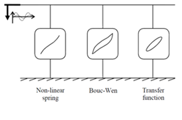
IPIT is used for the identification of the parameters of the Bouc-Wen and the numerator and denominator coefficients of the TFSISO element out of given measurement data.
Static Spline (Non-linear spring)
The non-linear spring is dedicated to capture the non-linear effects that appear at the large deflection amplitudes caused by the non-uniform shape of the bushing. In general the gradient at small and medium amplitudes is linear and therefore has a small influence on the amplitude dependency in this range. In addition, this element is used for introducing a preload force on the bushing.
The data of the static spline is not calculated in the parameter identification process, but is a required input. The data should be the result of a low frequency and high amplitude test. In other words, the user has to supply the backbone of the quasi-static test curve of the bushing.
TFSISO numerator and denominator coefficients
This part is dedicated to describe the frequency dependency of rubber bushings in terms of dynamic stiffness and loss angle. The impedance transfer function is used in the default template. See TFSISO section for more information.
Bouc-Wen hysteresis model
The Bouc-Wen hysteresis element is used to model the amplitude dependency at 'small' amplitudes of the excitation. In IPIT there are three versions of the hysteresis model: the coupled, the uncoupled and the revised version.
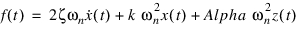
In all the Bouc-Wen versions, the hysteretic non-dimensional displacement, z, is described by the following non-linear differential equation, with zero initial condition, z(0)=0:

where:
■a is the parameter controlling hysteresis amplitude
■β, γ, n are the three parameters controlling hysteresis shape
Uncoupled version [BUSHING_COUPLING=0]
where:
■Alpha is the rigidity ratio
■ζ is the linear elastic viscous damping ratio
■ωn is the pseudo-natural frequency of the system
■k is the linear force scale
Coupled version [BUSHING_COUPLING=1]

where:
■Alpha is the rigidity ratio
■ζ is the linear elastic viscous damping ratio
■ωn is the pseudo-natural frequency of the system
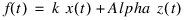
Revised version [BUSHING_COUPLING=2]

where:
■Alpha is the linear Bouc-Wen force scale
■k is linear force scale
■Note that ωn and ζ are not used in this version
Corrected version [BUSHING_COUPLING=3]
where:
■Alpha is the linear Bouc-Wen force scale
■k is linear force scale
■Note that ωn and ζ are not used in this version
Note: | BUSHING_COUPLING=3 is using the same equations as BUSHING_COUPLING=2, but has a correction for the rotational direction of the general bushing. |
General Bushing Measurement Data
The mathematical model has 6 parameters which are related to the amplitude dependency and 5 to 7 related to the frequency dependency. Taking into account that one measured point (frequency and amplitude) supplies two values, dynamic stiffness and loss angle, it is obvious that at least 3 measured amplitudes and 4 measured frequencies (for each measured amplitude) are required to achieve an exact mathematical solution.
Static Spline
The backbone of the quasi-static test loop of a bushing is used for determining the non-linear spline data. The measured (deflection) range should cover the operation range of the bushing (sometimes more than 8 mm). The measurements have to be performed including the preload.
Dynamic Data
The inputs of the model are amplitude and frequency while the outputs are dynamic stiffness and loss angle. The measured points, in frequency and amplitude range, of dynamic stiffness and loss are limited up to 128 points.
The data supplied must be in a squared matrix format. The number of frequency points of each amplitude should be identical. For example:
Amplitude | Frequency |
|---|---|
0.1 | 5 |
0.1 | 10 |
0.1 | 15 |
0.2 | 5 |
0.2 | 10 |
0.2 | 15 |
It is suggested to use the smallest possible number of points which can describe both amplitude and frequency response sufficiently for minimizing the computation time.
Deactivating a bushing direction
It is not required to provide bushing test data for every direction. The hysteresis and/or frequency dependent effect in a particular direction can be deactivated using the scaling factors:
$-------------------------------------------------------HYST_SCALES
[HYST_SCALES]
X_HYST_SCALE = 1.0
Y_HYST_SCALE = 1.0
Z_HYST_SCALE = 1.0
TX_HYST_SCALE = 1.0
TY_HYST_SCALE = 1.0
TZ_HYST_SCALE = 1.0
$-----------------------------------------------------TFSISO_SCALES
[TFSISO_SCALES]
X_TFSISO_SCALE = 1.0
Y_TFSISO_SCALE = 1.0
Z_TFSISO_SCALE = 1.0
TX_TFSISO_SCALE = 1.0
TY_TFSISO_SCALE = 1.0
TZ_TFSISO_SCALE = 1.0
For example, when setting the TX_HYST_SCALE and TX_TFSISO_SCALE to zero, the hysteresis (Bouc Wen) and TFSISO elements will not be used. The bushing force will be determined by the load-deflection curve (TX_CURVE) only.
Identification Process for General Bushings
The Adams Car Ride Isolator Parameter Identification Tool (IPIT) allows you to identify parameters of the general bushing, model out of measurement data. The IPIT can identify bushing parameters for each direction for which data is supplied in the GBU. The resulting bushing property file *.gbu can be used in for instance Adams Car for further study.
Following steps explain how to identify bushing parameters using the IPIT:
Step one: Prepare the .gbu property file for use with the IPIT
To avoid confusion with the *.gbu files, general bushing property file can be used in an Adams Car Assembly to calculate the bushing force but can also be used in IPIT for parameter identification of the bushing parameters out of measurement data. The headings marked below with (**) are used in IPIT during the identification only, this data is not used by Adams Solver.
The following shows all the parameters that must be defined in the GBU property file:
[MDI_HEADER]
■Specify the type, version and the format of the property file.
■Default: FILE_TYPE = 'gbu'
FILE_VERSION = 2.0
FILE_FORMAT = 'ASCII'
FILE_VERSION = 2.0
FILE_FORMAT = 'ASCII'
[UNITS]
■Specify the units of the test data under this block.
■Default: For IPIT the units are fixed to respectively:
LENGTH = 'millimeter'
FORCE = 'newton'
ANGLE = 'degrees'
MASS = 'kilogram'
TIME = 'second'
FORCE = 'newton'
ANGLE = 'degrees'
MASS = 'kilogram'
TIME = 'second'
[GENERAL]
DEFINITION is always '.aride.attachment.ac_general_bushing'
BUSHING_SHAPE=0/1/2/3
■Only the rectangular coupling is supported in IPIT.
■0 or 1 is rectangular coupling, 2 is cylindrical coupling and 3 is spherical coupling
■Default: to '0', this field is optional for IPIT.
BUSHING_COUPLING=0/1/2/3
■There are four versions of Bouc-Wen hysteresis model: the coupled, uncoupled and revised version.
■For the uncoupled version select 0, for the coupled select 1 and for the revised version select 3 (do not use version 2 because it contains a mistake in rotational direction).
■Default is '3', as the latest version of IPIT is developed for using this version.
■Not applicable for the g-direction.
[DAMPING]
■This field can be used to specify linear damping. It is suggested to use this parameter only when no Hysteresis (Bouc-Wen or TFSISO) model is used.
■There are 6 sets of damping parameters one for each coordinate (x/y/z/ax/ay/az).
■Default: '0.0', this block is optional.
[PRELOAD]
■This field can be used to modify the preload. It is suggested to modify the static spline instead of this parameter.
■There are 6 sets of preload parameters one for each coordinate (x/y/z/ax/ay/az).
■Default: '0.0', this block is optional.
[OFFSET]
■This field can be used to modify the offset of the static spline. It is suggested to modify the static spline instead of using this parameter.
■There are 6 sets of offset parameters one for each coordinate (x/y/z/ax/ay/az).
■Default: '0.0', this block is optional.
[SPLINE_SCALES]
■These scales are used by IPIT mainly as a switch to enable or disable the Static Spline component of the Bushing model. These can also be used in user defined strategies with the CMD export method.
■There are 6 sets of spline scale parameters one for each coordinate (x/y/z/ax/ay/az).
■Default: 1.0, so the Static Spline component of the Bushing model is enable. This block is compulsory.
[HYST_SCALES]
■These scales are used by IPIT as a switch to enable or to disable the Hysteresis / Bouc-Wen component of the Bushing model. These can also be used in user defined strategies with the CMD export method.
■There are 6 sets of hyst scale parameters one for each coordinate (x/y/z/ax/ay/az).
■Default: For the Translation directions, default is 1.0, for the rotational direction the default is 57.295 (=180/pi). When the Hysteresis/Bouc-Wen component of the Bushing model is enabled, this block is compulsory.
[TFSISO_SCALES]
■These scales are used by IPIT as a switch to enable or to disable the TFSISO component of the Bushing model. These can also be used in user defined strategies with the CMD export method.
■There are 6 sets of tfsiso scale parameters one for each coordinate (x/y/z/ax/ay/az).
■Default: For the Translation directions, default is 1.0, for the rotational direction the default is 57.295 (=180/pi). When the TFSISO component of the Bushing model is enabled, this block is compulsory.
[FX/ FY/ FZ/ TX/ TY/ TZ _CURVE]
■This block contains the Spline Curves data.
■There are 6 sets of Spline Curves parameters one for each coordinate (x/y/z/ax/ay/az).
■No default values and it is compulsory only for the identifying direction.
[BUSHING_PARAMETERS]
■This block is used to supply bushing parameters for Bouc-Wen and TFSISO. While using in Adams Car Assembly and IPIT, the bushing force is calculated using these parameters. IPIT updates these data during the optimization process.
■There are 6 sets of bushing parameters one for each coordinate (x/y/z/ax/ay/az).
■Default: (valid for the revised version of the Bouc-Wen model).
The lower default values could be used, but for the BUSHING_COUPLING = 3 model, the optimizer is able to generate good starting values automatically.
Parameter | Default Value |
|---|---|
Alpha | It is suggested to put the average dynamic stiffness of all the measured amplitude range at the lowest frequency |
Beta | 1.7 |
Gamma | 0.2 |
Zeta | 0.0 - it is not used in the revised version of Bouc-Wen |
Omega | 0.0 - it is not used in the revised version of Bouc-Wen |
a | 1.0 |
n | 0.2 |
K | 0.0 |
Num | [0.0,0.0] |
Den | [0.0,1.0] |
[BUSHING_TEST_DATA_X/Y/Z/AX/AY/AZ] (**)
■This block contains four columns of data, the dynamic measuring data of the bushing corresponding to the direction X, Y, Z, AX, AY and AZ. As it is discussed in the General Bushing Measurement Data section, all measured amplitudes should have the same number of measured frequencies.
■At least one block with test data is compulsory for the operation of IPIT.
■Input format: the supplied matrix should have the following columns, always in this listed order:
{amplitude frequency cdyn phase scale}
[BUSHING_IDENTIFICATION_DATA_X/Y/Z/AX/AY/AZ] (**)
■This block contains a matrix with exactly the same dimensions as the BUSHING_TEST_DATA_X/Y/Z/AX/AY/AZ block. These are the dynamic stiffness and phase data calculated by the bushing model with the identified parameters.
■Default: This is an optional block. In general the dynamic stiffness and loss angle data is added by IPIT after each optimization process.
Step two: Set-up the IPIT for the bushing parameter identification process
Best optimization process is available for bushings with BUSHING_COUPLING=3, then the latest version of the bushing model is used, and the optimization is done in steps, improving convergence, stability, performance and accuracy. The following steps are used:
1. TFSISO (freq. domain)
First the optimization tool will calculate the parameters of the transfer function (TFSISO) only using a Maxwell or Frequency Bushing model (Start Method TFSISO) for having sufficient constraints for the optimization process. This optimization is done in frequency domain (fast) and neglects the values for the Bouc-Wen.
2. TFSISO & BW (freq. domain)
Next the optimization tool will further optimize the parameters of the transfer function (TFSISO) and add the effect of the Bouc-Wen function (BW) in frequency domain. The start values for the Bouc Wen can be either estimated from the Bushing data (Start Values BW), or the values from the GUI can be taken.
To verify the accuracy of the frequency domain results in the time domain using test rig simulations, the user can click on the 'Calculate Frequency Response w Test Rig Simulations'. If differences are large and not acceptable, a third step in the optimization can be executed.
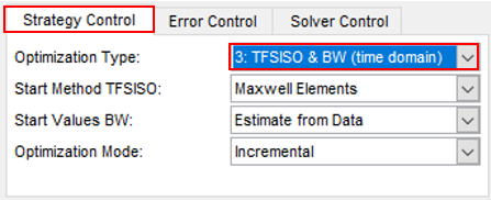
3. TFSISO & BW (time domain)
As last step, the optimization tool will further improve the parameters of the transfer function (TFSISO) and the Bouc-Wen function (BW) in the time domain using bushing test rig simulations (time domain).
When using the following setting of the strategy control, the first 2 steps will be executed. These optimizations are done in frequency domain and fast.
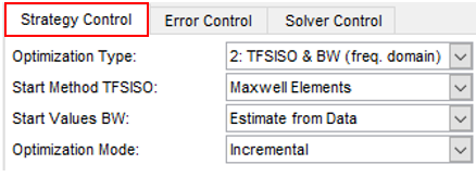
After these two steps, one can verify the accuracy in the time domain by clicking on

If further optimization is required, the third step (optimization in time domain) can be executed:
It is also possible to change parameters in the gui manually and verify the effect of the change by clicking on one of the 'Calculate Frequency Response' buttons. Step 3 will always that the actual values from the gui in case of Single Optimization Mode.
An example general bushing file is the <aride_shared>/general_bushing.tbl/gen_bus003.gbu.
Note: | When optimizing a general bushing for one of the rotational directions with a BUSHING_COUPLING < 3, the rotational scale factors need to be set to 57.29577951. [HYST_SCALES] X_HYST_SCALE = 1.0 Y_HYST_SCALE = 1.0 Z_HYST_SCALE = 1.0 TX_HYST_SCALE = 57.29577951 TY_HYST_SCALE = 57.29577951 TZ_HYST_SCALE = 57.29577951 $----------------------------------TFSISO_SCALES [TFSISO_SCALES] X_TFSISO_SCALE = 1.0 Y_TFSISO_SCALE = 1.0 Z_TFSISO_SCALE = 1.0 TX_TFSISO_SCALE = 57.29577951 TY_TFSISO_SCALE = 57.29577951 TZ_TFSISO_SCALE = 57.29577951 |
For property files with BUSHING_COUPLING not equal to 3 and hydro mount property files (.hbu) just the third optimization type (time domain optimizations) can be performed.
The effect of the Offset and Preload
The 'Offset' in the IPIT dialog window allows you to specify another working position of the general bushing at load-deflection curve (FX_CURVE, FY_CURVE, FZ_CURVE, TX_CURVE, TY_CURVE, TZ_CURVE). If the load-deflection curve is linear, there will be no effect on the dynamic stiffness, but with a non-linear load-deflection curve the dynamic stiffness and damping will change.
A preload will not change the dynamic stiffness and damping, because the static force will not have a dynamic effect.
The effect of the mount inertia
Depending on the measurement data, the inertia of the bushing mounts may be included or not included (corrected) in the measurement data. If not included the 'Include Mount Inertia' radio button setting must be changed. For hydromount data, the inertia of the mounts is not taken into account in the IPIT fitting by default.
The IPIT will show the parameters of the property file [HYDRO_PARAMETERS], plot the bushing test data points from the [HDYRO TEST DATA] section and then draw the lines in between the [HYDRO IDENTIFICATION DATA] data points. These last points have generated by the hydromount model using the hydromount parameters.
IPIT Optimizer
The IPIT works with the MPFit optimizer:
MPFit aims for minimizing the sum of the squares of m nonlinear functions in n variables by the Levenberg- Marquardt algorithm. With the IPIT the MPFit is used to minimize the difference in between the bushing dynamic stiffness and loss angle data point and the dynamic stiffness and loss angle calculated by the general bushing or hydromount model.
Constraints
In general the default constraints (limits for each parameter per Optimization Type) for the general bushing parameters can be used. However in a special case, one may want to change the constraints, they are defined in an external file: <adams_installation_directory>/aride/ shared_ride_database.cdb/general_bushing.tbl/ipit_par_constraints.txt.
If one wants the IPIT to use another file with constraints definitions (not to change the generic constraints file), the environment variable MSC_IPIT_CONSTRAINTS_FILE can be defined with an alternative path and name (before starting Adams) for the constraints, for example:
MSC_IPIT_CONSTRAINTS_FILE=d:/adams/my_constraints.txt
Running IPIT in Batch Mode
By using the File - Export CMD option, command scripts can be prepared to run the IPIT in batch mode:
1. Load the .gbu or .hbu property file that has the bushing test data that needs to be processed by the optimizer.
2. Set the options to be used for the optimizer, for example, Optimization Type 3, Start Method TFSISO, Start Values BW or Optimization Mode.
3. Export the CMD
4. The cmd can be run from the Adams Car in interactive model. Start Adams Car, click on File → Import and then select the created cmd file.
Or can be run in batch mode with following commands:
Windows:
adams2024_1 acar ru-acar b <your cmd script name>.cmd exit
Linux:
adams2024_1 -c acar ru-acar b <your cmd script name>.cmd exit
Running IPIT with Bushing in 'g'-direction
When loading the file <top_dir>/aview/examples/bushings/gen_bus002.gbu, the IPIT will start in g-direction as shown below.
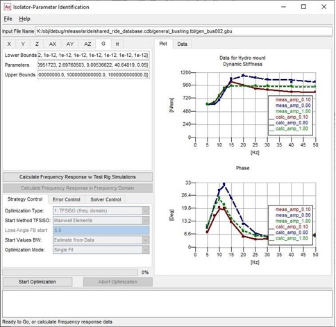
Note: | In the Strategy Control tab, only Step 3: optimization is available (optimization in time domain with test rig simulations). |
By changing the bushing_template (see below), the optimization of any bushing can be done with the IPIT as long as the number of parameters does not exceed 128.
Modify the Bushing Template File
The IPIT uses a python template file to calculate the bushing response using Adams Solver (C++). This python template file contains Adams Solver .acf and .adm files. You can modify the Adams Solver statements and add for instance your own user libraries for bushings in this template. The example python template file is located in: adams_install/python/Arch/Lib/site-packages/bushing_templates.py, where Arch is your platform (win64, linux64 and so on.) and install is your Adams installation folder. If you open the template file, you will find a number of template variables including description at the beginning of this file. You may study the example template to understand how the template variables are used to create a bushing model used in combination with the IPIT. Modification of the template file allows you to include your own bushing model. The IPIT uses two important python string variables acftext and admtext to recognize your ADM and ACF templates.
The example python template file has one .acf template and two .adm sample templates. The admtext python string variable lists the .adm template for the Adams general bushing which is used by the IPIT to identify the general bushing parameters (example template file for BUSHING_COORDINATE = 'x' or 'y' or 'z' or 'ax' or 'ay' or 'az' or 'g' or 'h').
The python template file can contain multiple ACF and ADM templates, but the IPIT only uses the template represented by the python string variables acftext and admtext.
It is also possible to create a customized python template and hook-up it to the IPIT by defining environment variable IPIT_TEMPLATE_PATH. The user template file name is restricted to 'user_bushing_templates.py' and it should reside in the directory referred by environment variable IPIT_TEMPLATE_PATH (for example, IPIT_TEMPLATE_PATH=C:/users/IPIT_user_dir). If the path or file is not accessible or incorrect, IPIT uses the default template from the installation, which is the template for the Hydromount bushing. IPIT also informs the user about which template it is using by printing a message in the command shell.