Example of Modal Loads
Overview
In this tutorial, you’ll explore how a steel plate, shown in Figure 1, responds to the distributed loads listed below. The steel plate is 1 meter square and 10 mm thick. It is supported vertically at all four corners and restrained against rotation in its plane.
■Uniform pressure - An overpressure of one atmosphere (atu) uniformly applied on the top surface.
■Centered pressure - An overpressure of one atu applied to a .4 M by .4 M square on the plate center.
■Parabolic pressure - An overpressure parabolically varying in the normal direction only, from a value of zero at the edge to one atu in the center.
You’ll apply the loads by creating a modal force in Adams View. You’ll then run a dynamic simulation to see how the first loadcase (uniform pressure) alters the plate over time. You’ll then see the effects of disabling some of the modes and find the static equilibrium of the forces and plate flexibility. Finally, you’ll run simulations using the other loadcases.
Each time you run a simulation, you’ll review the results in Adams PostProcessor to see how they compare to similar data obtained from MSC.Nastran.
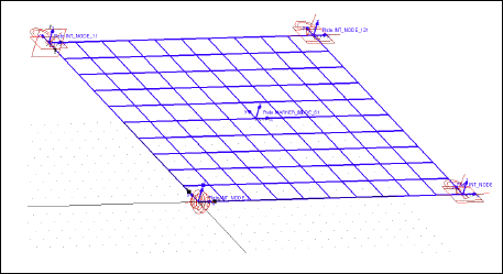
Figure 1 Steel Plate
Correlation with MSC.Nastran Data
For each of the applied loads listed on page 1, we ran a MSC.Nastran static solution. Table 1 compares the MSC.Nastran and Adams static results for the plate center deflections and corner reaction loads. During the tutorial, you’ll compare the results that you obtain, with the results in the table.
Loadcase: | Static center deflection (M): | Corner reaction (N): | ||
|---|---|---|---|---|
MSC.Nastran | Adams | MSC.Nastran | Adams | |
Uniform pressure - | .12533 | -.12535 | +25335 | +25335 |
Centered pressure | -.02769 | -.02835 | +4053 | +4054 |
Parabolic pressure | -.09372 | -.09371 | +17125 | +17126 |
Note that Adams Flex has solved the problem using a reduced set of degrees of freedom (DOF). The Adams Flex solutions, therefore, do not match the MSC.Nastran solution exactly.
About the Tutorial Files
We’ve included three files to define the plate and the loads applied to it:
■plate.cmd - This file contains Adams View commands that create a model called Simple and integrate into the model a flexible body called Plate. The commands also constrain the plate at all four corners using one spherical joint, two inplane joint primitives, and one inline joint primitive. Finally, they create a marker at the center of the plate from which to measure displacements.
■plate_load.mnf - This file defines the flexible body and associates the loadcases in plate.loads with the flexible body. The file plate.cmd reads in this file.
■Before giving you this file, we used the tool mnfload to associate a loadcase file, plate.loads, with the flexible body. This loadcase file defines the three sets of loadcases for the plate. It is an ASCII file that lists the loads to be applied at each node. A comment that begins with a %C separates the different loadcases in the file. Adams View stores the comments as titles for the loadcases so you can select the ones you want to apply.
Starting Adams View
You’ll start the tutorial by running Adams View and importing the command file, plate.cmd, to create a model called Simple.
To start Adams View and create a model:
1. Copy the file plate.cmd and plate_load.mnf to your local directory. This file is located in install_dir/flex/examples/mnfload, where install_dir is the directory where the Adams software is installed.
2. Start Adams View and import the command file plate.cmd.
Adams View starts and the steel plate appears, as shown in Figure 1.
3. Rotate the plate so you can see it more easily (that is, not from directly above).
Creating a Measure
In this section, you create a point-to-point measure that measures the plate deformation at the center of the plate.
To create the measure:
 .
. 2. In the container on the Main toolbox, set Component to Global Z.
3. Following the instructions in the status bar, select marker_22 as the location from which to measure.
4. Select Plate.MARKER_NODE_61 as the location to which to measure.
Creating a Modal Force to Apply the Distributed Loads
Now you’ll create a modal force (MFORCE) in Adams View to apply the distributed loads to the plate. You’ll apply the load in the first loadcase, called one atu overpressure, which applies a uniform pressure on the plate.
To create a modal force:

The Create Modal Force dialog box appears. Notice that the loadcase information does not appear in the dialog box. This is because you have not specified a flexible body yet.
2. In the Flexible Body text box, enter Plate.
Adams View automatically enters the names of the loadcases associated with the flexible body Plate into the Load Case option menu.
3. Set Load Case to one atu overpressure.
4. In the Scale Function text box, enter a function to vary the pressure over time. In this case, enter the function:
sin(PI*time)
5. Select OK.
Adams View displays a MFORCE icon at the lower left corner (LPRF) of the plate.
Simulating the Distributed Loads
Now you’ll run a dynamic simulation to see how Adams Flex applies the loads over time.
To run a dynamic simulation:
 .
. 2. Set End Time to 1.0 and Steps to 50.
3. Select the Simulation Start tool.
You see the plate deform as Adams Flex applies the loads.
Reviewing the Results of the Simulation
You’ll now review the results of the simulation, which include:
■Point-to-point measure to see how the location of the center of the plate (Node 61) changed relative to marker_22.
■Reaction forces (FZ) at the corners of the plate.
■Modal forces of the various modes (FQ). The sum of all the modes equals the applied force.
To review the results of the measure:
1. From the Review menu, select PostProcessing.
Adams PostProcessor appears.
2. Set Source to Measures.
3. From the Measure list, select MEA_PT2PT_1, and then select Add Curves.
The plot shows the time history of the plate center deflection.
4. Compare the maximum deflection that Adams Flex returned, with the maximum deflection from MSC.Nastran, listed in Figure 1. Notice that the Adams Flex deflection is slightly larger in magnitude because it contains a small dynamic component that is not present in the MSC.Nastran solution. You will compute the static solution later in the tutorial (Running a Time-Independent (Static) Simulation.)
To review the results of the reaction forces:
1. From the dashboard in Adams PostProcessor, set Source to Objects.
2. From the Filter list, select constraint.
3. From the Object list, select one of the joints that holds the plate in place. For example, select Joint_4, the spherical joint in the lower left corner of the plate.
4. From the Characteristic list, select Element_Force.
5. From the Component list, select Z.
6. Select Surf.
7. Continue selecting joints and their reaction force. You will notice that the reaction forces are the same for all joints.
8. Compare the reaction forces with the forces obtained from MSC.Nastran shown in Table 1. Again, the dynamic results differ from the static results.
To review the modal forces:
1. From the dashboard in Adams PostProcessor, set Source to Result Sets.
2. From the Result Set list, select MFORCE_1.
3. From the Component list, select any modal force component. The modal force components are listed as FQn, where n is the number of the mode. Note that most of the modes have zero contributions, whereas a few of the modes (9, 14, 20, 25, and 36) have non-zero contributions.
For Adams Flex to accurately model this particular distributed load on the plate, each of these modes needs to be enabled. If one of these modes is disabled, its contribution to the modal force is not included in the simulation. You’ll see the effects of this in the next section.
4. When you are done, from the File menu, select Close Plot Window to return to the Adams View main window.
Viewing Effect of Disabling Modes
Now you’ll disable modes 20 to 48. You’ll then run another dynamic simulation to see the effects of disabling modes on the maximum deflection of the plate center and to see how the reaction forces at the joints compare to the previous simulation. The point-to-point measure calculates the plate center deflection.
To disable modes:

2. Display the Flexible Body Modify dialog box.
3. Select range.
4. In the Enable or Disable a Range of Modes dialog box, set the options to disable all modes above 19 based on mode number.
5. Select OK.
To run a simulation:
■Run the simulation using the same values as before (Dynamic, one second, and 50 steps).
To review the results:
1. Follow the instructions in Reviewing the Results of the Simulation on page 6, to review the point-to-point measure and joint forces.
2. As you review them, notice that the maximum deflection of the plate center is significantly smaller (approximately 8 to 10% smaller), now that you’ve disabled the modes. Note, however, that the sum of the reaction forces remains the same.
In the previous section of this tutorial, you found that modes 20, 25, and 36 contributed significantly to the associated distributed load. Because you disabled these modes in this section, modal load truncation occurred, resulting in a smaller deflection of the plate.
The resulting reaction forces on the joints were barely affected by the modal truncation because Adams Flex derives them from the forces and torques associated with flexible body’s six rigid body degrees of freedom. These six forces and torques represent the external resultant of the distributed loadcase projected by all of the modes during the MNF to matrix translation.
Running a Time-Independent (Static) Simulation
In this section, you’ll modify the modal force so it is constant over time and perform a static equilibrium simulation, comparing the results with MSC.Nastran results.
To modify the MFORCE:
1. Right-click the MFORCE icon. From the shortcut menu that appears, point to the modal forces, and then select Modify.
The Modify Modal Force dialog box appears.
2. In the Scale Function text box, remove the function and enter 1.0.
3. Select OK.
Enable the modes:
1. Display the Flexible Body Modify dialog box.
2. Select range and enable all the non-rigid body modes (7 through 48).
To run a static equilibrium:
2. Select the Static Equilibrium tool. 
To review the results:
1. Review the strip chart of the measure by noting the value in the legend.
2. Compare the static displacement of the plate center with those obtained from MSC.Nastran, shown in Table 1.
Simulating Remaining Loadcases
Now go ahead and run Adams simulations of the remaining two loadcases:
■Centered pressure - An overpressure of one atu applied to a .4 M by .4 M square on the plate center.
■Parabolic pressure - An overpressure parabolically varying in the x-direction only, from a value of zero at the edge to 1 atu in the center.
To run the simulations:
1. Modify the modal force so it refers to one of the loadcases listed above.
2. Perform a static simulation.
3. Compare with the values in Table 1.