Modal flexibility in Adams
In this section we show how Adams capitalizes on modal superposition in the two key areas of the Adams formulation:
■Flexible marker kinematics
■Flexible body equations of motion
Flexible Marker Kinematics
Marker kinematics refers to the position, orientation, velocity, and acceleration of markers. Adams uses the kinematics of markers in three key areas:
■Marker position and orientation must be known in order to satisfy constraints like those imposed in JOINT and JPRIM elements.
■To project point forces applied at markers on generalized coordinates of the flexible body.
■The marker measures, (for example DX, WZ, PHI, ACCX, and so on) that appear in expressions and user-written subroutines require information about position, orientation, velocity, and acceleration of markers
Position
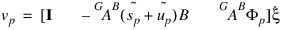
The instantaneous location of a marker that is attached to a node,  , on a flexible body,
  , is the sum of three vectors (see Figure 7).
, on a flexible body, , is the sum of three vectors (see Figure 7).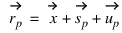 | (24) |
where:
 | = | the position vector from the origin of the ground reference frame to the origin of the local body reference frame,  , of the flexible body. , of the flexible body. |
 | = | the position vector of the undeformed position of point  with respect to the local body reference frame of body with respect to the local body reference frame of body  . . |
 | = | the translational deformation vector of point  , the position vector from the point’s undeformed position to its deformed position , the position vector from the point’s undeformed position to its deformed position |
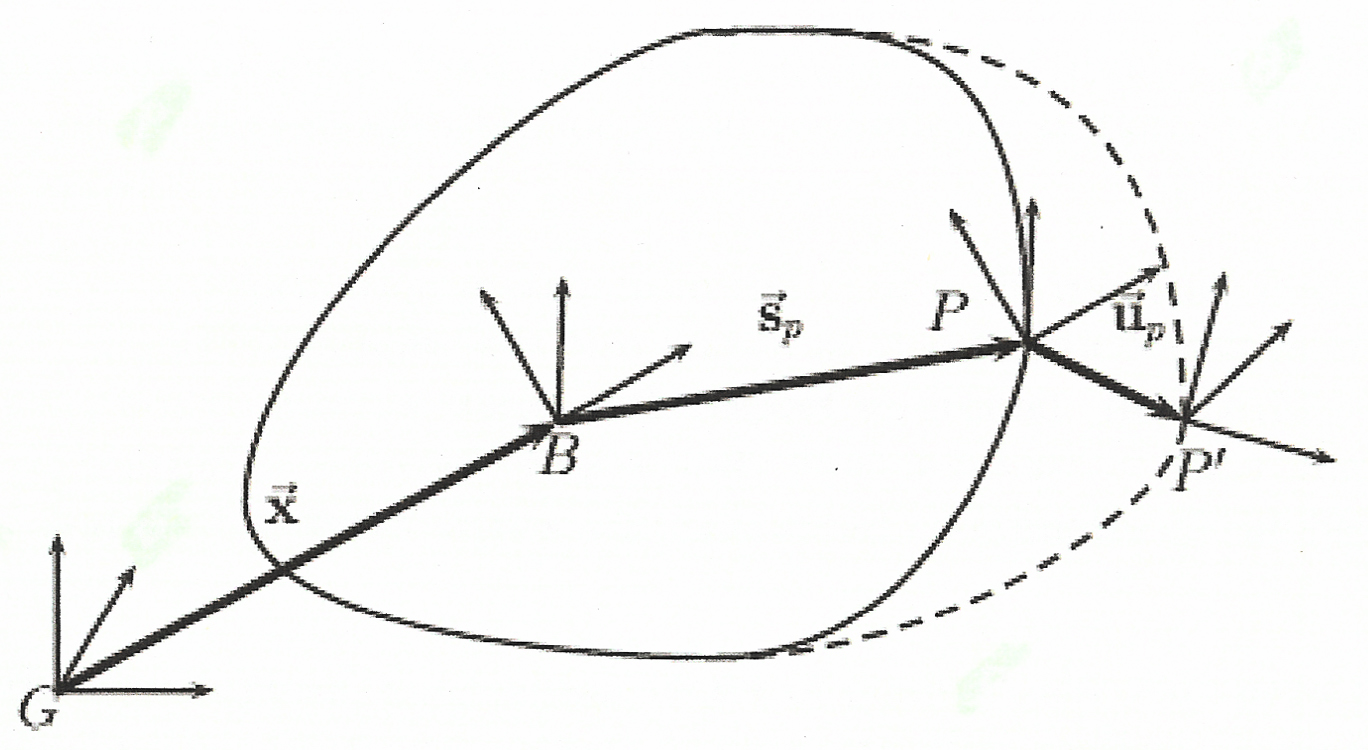
Figure 7 The position vector to a deformed point  on a flexible body relative to a local body reference frame
  and ground
on a flexible body relative to a local body reference frame and ground We rewrite Equation (24) in a matrix form, expressed in the ground coordinate system
 | (25) |
where:
 | = | the position vector from the ground origin to the origin of the local body reference frame,  , of the flexible body, expressed in the ground coordinate system. The elements of the , of the flexible body, expressed in the ground coordinate system. The elements of the  vector, x, y and z, are generalized coordinates of the flexible body. vector, x, y and z, are generalized coordinates of the flexible body. | ||
 | = | the position vector from the local body reference frame of  to the point to the point  , expressed in the local body coordinate system. This is a constant. , expressed in the local body coordinate system. This is a constant. | ||
 | = | the transformation matrix from the local body reference frame of  to ground. This matrix is also known as the direction cosines of the local body reference frame with respect to ground. In Adams, orientation is captured using a body fixed 3-1-3 set of Euler angles, to ground. This matrix is also known as the direction cosines of the local body reference frame with respect to ground. In Adams, orientation is captured using a body fixed 3-1-3 set of Euler angles,  , ,  and and  . The Euler angles are generalized coordinates of the flexible body. . The Euler angles are generalized coordinates of the flexible body. | ||
 | = | the translational deformation vector of point  , also expressed in the local body coordinate system. The deformation vector is a modal superposition. , also expressed in the local body coordinate system. The deformation vector is a modal superposition.
where  is the slice from the modal matrix that corresponds to the translational DOF of node is the slice from the modal matrix that corresponds to the translational DOF of node  . The dimension of the . The dimension of the  matrix is matrix is  where where  is the number of modes. The modal coordinates is the number of modes. The modal coordinates  , ,  are generalized coordinates of the flexible body. are generalized coordinates of the flexible body. |

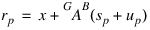
Therefore, the generalized coordinates of the flexible body are:
 | (27) |
Velocity
For the purpose of computing kinetic energy, we compute the instantaneous translational velocity of  relative to ground which is obtained by differentiating Equation (25) with respect to time:
relative to ground which is obtained by differentiating Equation (25) with respect to time: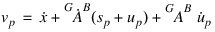 | (28) |
Taking advantage of the relationship:
 | (29) |
where  is the angular velocity of the body relative to ground (expressed in body coordinates with the tilde denoting the skew operator of Equation (34) we can write:
is the angular velocity of the body relative to ground (expressed in body coordinates with the tilde denoting the skew operator of Equation (34) we can write: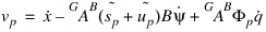 | (30) |
We have introduced the relationship:
 | (31) |
relating the angular velocity to the time derivative of the orientation states.
Orientation
To satisfy angular constraints, Adams must instantaneously evaluate the orientation of a marker on a Flexible body, as the body deforms. As the body deforms, the marker rotates through small angles relative to its reference frame. Much like translational deformations, these angles are obtained using a modal superposition, similar to Equation (26)
 | (32) |
where  is the slice from the modal matrix that corresponds to the rotational DOF of node
  . The dimension of the
  matrix is
  where
where  is the number of modes.
is the slice from the modal matrix that corresponds to the rotational DOF of node . The dimension of the matrix is where is the number of modes.The orientation of marker  relative to ground is represented by the Euler transformation matrix,
  . This matrix is the product of three transformation matrices:
relative to ground is represented by the Euler transformation matrix, . This matrix is the product of three transformation matrices: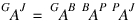 | (33) |
where:
 | = | the transformation matrix from the local body reference frame of  to ground. to ground. |
 | = | the transformation matrix due to the orientation change due to the deformation of node  . . |
 | = | the constant transformation matrix that was defined by the user when the marker was placed on the flexible body. |
The matrix  requires more attention. The direction cosines for a vector of small angles,
  , are:
requires more attention. The direction cosines for a vector of small angles, , are: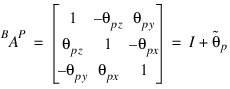 | (34) |
where the tilde denotes the skew operator:
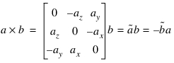 | (35) |
Angular velocity
The angular velocity of a marker,  , on a flexible body is the sum of the angular velocity of the body and the angular velocity due to deformation:
, on a flexible body is the sum of the angular velocity of the body and the angular velocity due to deformation: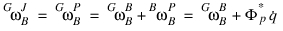 | (36) |
Applied loads
The treatment of forces in Adams distinguishes between point loads and distributed loads. This section discusses the following topics:
■Point forces and torques
■Distributed loads
■Residual forces and residual vectors
Point Forces and Torques
A point force  and a point torque
  that are applied to a marker on a flexible body must be projected on the generalized coordinates of the system.
and a point torque that are applied to a marker on a flexible body must be projected on the generalized coordinates of the system.The force and torque are written in matrix form, and expressed in the coordinate system of marker  .
.
.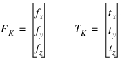 | (37) |
The generalized force  consists of a generalized translational force, a generalized torque (a generalized force on the Euler angles) and a generalized modal force, thus:
consists of a generalized translational force, a generalized torque (a generalized force on the Euler angles) and a generalized modal force, thus: | (38) |
Generalized Translational Force: Since the governing equations of motion, Equation (56), are written in the global reference frame, the generalized force on the translational coordinates is obtained by transforming  to global coordinates.
to global coordinates. | (39) |
where  is given in Equation (33). The generalized translational force is independent of the point of force application.
is given in Equation (33). The generalized translational force is independent of the point of force application.An applied torque does not contribute to  .
.
.Generalized Torque: The total torque on a flexible body, due to  and
and  is
is 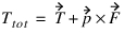 where
where  is the position vector from the origin of the local body reference frame of the body to the point of force application. The total torque, can be written in matrix form, with respect to the ground coordinate system as:
and is where is the position vector from the origin of the local body reference frame of the body to the point of force application. The total torque, can be written in matrix form, with respect to the ground coordinate system as: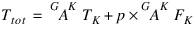 | (40) |
where  is expressed in the ground coordinates. Using the tilde notation of Equation (35), this can be written as:
is expressed in the ground coordinates. Using the tilde notation of Equation (35), this can be written as: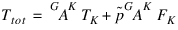 | (41) |
The transformation from torque in physical coordinates to the generalized torque on the body Euler angles is provided by the  matrix in Equation (31).
matrix in Equation (31). | (42) |
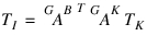
Generalized Modal Force: The generalized modal force on a body due to applied point forces or point torques at  is obtained by projecting the load on the mode shapes.
is obtained by projecting the load on the mode shapes.As the applied force  and torque
  are given with respect to marker
  , they must first be transformed to the reference frame of the flexible body:
and torque are given with respect to marker , they must first be transformed to the reference frame of the flexible body: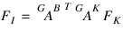 | (43) |
 | (44) |
and then projected on the mode shapes. The force is projected on the translational mode shapes and the torque is projected on the angular mode shapes:
 | (45) |
where  and
and  are the slices of the modal matrix corresponding to the translational and angular DOF of point
  , as discussed in Flexible Marker Kinematics.
and are the slices of the modal matrix corresponding to the translational and angular DOF of point , as discussed in Flexible Marker Kinematics.Note that since the modal matrix  is only defined at nodes, point forces and point torques can only be applied at nodes.
is only defined at nodes, point forces and point torques can only be applied at nodes.Distributed Loads
Although distributed loads can be generated in Adams as an array of point loads, this is rarely an efficient approach. As an alternative, distributed loads can be created in Adams using the MFORCE element. The MFORCE statement allows you to apply any distributed-load vector.
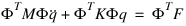
A discussion of distributed loads starts by examining the physical coordinate form of the equations of motion in the finite element modeling software.
 | (46) |
Here  and
and  are the FEM mass and stiffness matrices for the flexible component, and
  and
and  are, respectively, the physical nodal DOF vector and the load vector.
and are the FEM mass and stiffness matrices for the flexible component, and and are, respectively, the physical nodal DOF vector and the load vector. using the modal matrix
  :
: | (47) |
This modal form of the equation simplifies to:
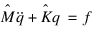 | (48) |
where  and
and  are the generalized mass and stiffness matrices and
  is the modal load vector.
and are the generalized mass and stiffness matrices and is the modal load vector.The applied force is likely to have a global resultant force and torque. These show up as loads on the rigid body modes and are treated in Adams as point forces and torques on the local reference frame, as covered in the previous section. The global resultant force and torque are not discussed further.
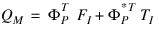
The projection of the nodal force vector on the modal coordinates:
 | (49) |
is a computationally expensive operation, which poses a problem when  is a arbitrary function of time. Adams circumvents this problem by introducing the simplifying assumption that the spatial dependency and the time dependency can be separated, i.e., that the load can be viewed as a time varying linear combination of an arbitrary number of static load cases:
is a arbitrary function of time. Adams circumvents this problem by introducing the simplifying assumption that the spatial dependency and the time dependency can be separated, i.e., that the load can be viewed as a time varying linear combination of an arbitrary number of static load cases: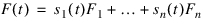 | (50) |
Then the expensive projection of the load to modal coordinates can be performed once during the creation of the MNF, rather than repeatedly during the Adams simulation. Adams need only be aware of the modal form of the load:
 | (51) |
where the vectors  to
to  are n different load case vectors. Each of the load case vectors contains one entry for each mode in the modal basis.
to are n different load case vectors. Each of the load case vectors contains one entry for each mode in the modal basis.A more generous definition of  allows it to have an explicit dependency on system response, which we will denote as
  , where
  now represents all the states of the system, not just those of the flexible body. The equation for the modal force can now be written as:
allows it to have an explicit dependency on system response, which we will denote as , where now represents all the states of the system, not just those of the flexible body. The equation for the modal force can now be written as: | (52) |
Residual Forces and Residual Vectors
Implicit in the discussion in the previous sections is the assumption that the modal projection of the applied force:
 | (53) |
is exhaustive. However, due to mode truncation, in practice this is not always the case. In some cases, some amount of force remains unprojected. We refer to this force as the residual force. One might think about this as the load that was projected on the neglected higher-order modes.
The value of the residual force could be evaluated as:
 | (54) |
Associated with a residual force is residual vector, which can be thought of as the deformed shape of the flexible body when the residual force is applied to it. This residual vector can be treated as a mode shape and added to the (CMS) modal basis. This enhanced basis completely captures the applied load. Without this enhancement, the residual force is irretrievably lost.
There are two load cases where residual force is not a concern:
■Point forces or torques on CMS boundary nodes. The nature of the component modal synthesis (CMS) modal basis is such that point loads on the boundary nodes project perfectly on the corresponding constraint modes.
■Uniform distributed loads. Uniform distributed loads project completely on the rigid body DOFs.
There is one special case of force truncation that deserves mention. This case is best illustrated by considering a FEM node with incomplete stiffness, as found on solid elements or shell elements. Applying a load to this node leads to a singularity in the FEM analysis. When CMS modes are generated for this model, they will share a common attribute--the mode shape entry for this DOF is zero in all the modes. Consequently, any attempts in Adams to apply a load in this DOF will fail, because the load does not project on any of the modes and the structure will appear infinitely stiff. It is recommended that no loads be applied in Adams that could not have been applied in the FEM software.
Preloads
Adams supports preloaded flexible bodies. This allows Adams to support non-linear FEM analyses by accepting flexible bodies that have been linearized in a deformed state. These modes would not otherwise be considered candidates for a modal representation in Adams.
However, in certain Adams analyses the deformations of the non-linear component might safely be assumed to remain within a small range around a fixed operating point and a linearization of the body about this operating point could yield a useful modal representation of the body. A non-linear finite element model of the body is brought to this operating point by applying some combination of loads. The body is linearized at the operating point and the modes are extracted and exported to Adams.
Figure 8 Force Deformation plot
Figure 8 illustrates the force-deformation relationship of the process described above. The undeformed state is defined by operating point  . As the body deforms, it is brought through a non-linear path to a deformed state
  . A linear model of the body at
  , such as might have been defined by an Adams flexible body, would incorrectly have predicted an operating point at
  rather than at
  . Note further, that if the body is linearized at
  , and a modal description exported to Adams in the form of a preloaded flexible body, a limited range of validity must also be observed. Fully unloading the Adams flexible body would bring it to operating point
  , which is not correct.
. As the body deforms, it is brought through a non-linear path to a deformed state . A linear model of the body at , such as might have been defined by an Adams flexible body, would incorrectly have predicted an operating point at rather than at . Note further, that if the body is linearized at , and a modal description exported to Adams in the form of a preloaded flexible body, a limited range of validity must also be observed. Fully unloading the Adams flexible body would bring it to operating point , which is not correct.A preload is applied in Adams in the same way modal loads described in the previous section are applied, except that the preload is not under the user’s control. The preload cannot be disabled or scaled because it is considered an immutable property of the flexible bodies with an associated deformed geometry. Only one preload can be defined for any given flexible body.
A preload is an internal load and as such only operates on the modal coordinates. There is no global resultant force. In other words, there is no load on the rigid body DOF. If this were otherwise, the flexible body would have a tendency to accelerate itself, which would be counterintuitive.
Unless the external load that gave rise to the preload is reapplied within Adams, the preloaded flexible body will recoil. If the flexible body originated from a linear finite element model, it will recoil to its undeformed shape. If the body came from a non-linear analysis, the effect will be more like that described in Figure 8. If the body is constrained to other bodies, this tendency to recoil will cause the body to push on the other bodies.
Flexible Body Equations of Motion
The governing equations for a flexible body are derived from Lagrange’s equations of the form:
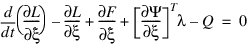 | (55) |
 | (56) |
where:
 | = | the Lagrangian, defined below. |
 | = | an energy dissipation function, defined below. |
 | = | the constraint equations. |
 | = | the Lagrange multipliers for the constraints. |
 | = | the generalized coordinates as defined in Equation (27). |
 | = | the generalized applied forces (the applied forces projected on  ). ). |
The Lagrangian is defined as:

where  and
and  denote kinetic and potential energy respectively.
and denote kinetic and potential energy respectively.The remainder of this section is devoted to the derivation of the contributions to Equation (56), in the following order:
■Kinetic energy and the mass matrix.
■Potential energy and the stiffness matrix.
■Dissipation and the damping matrix.
■Constraints.
Kinetic Energy and the Mass Matrix
The velocity from Equation (30) can be expressed in terms of the time derivative of the state vector  :
:
: | (57) |
We can now compute the kinetic energy. The kinetic energy for a flexible body is given as:
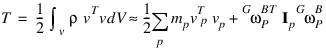 | (58) |
where  and
and  are the nodal mass and nodal inertia tensor of node
  , respectively. Note that
  is often a negligible quantity which arises when reduced continuum descriptions, i.e. bars, beams, or shells, are employed in your flexible component model. Lumped masses and inertia may also contribute to this term.
and are the nodal mass and nodal inertia tensor of node , respectively. Note that is often a negligible quantity which arises when reduced continuum descriptions, i.e. bars, beams, or shells, are employed in your flexible component model. Lumped masses and inertia may also contribute to this term.Substituting for  and
and  and simplifying yields an equation for the kinetic energy in Adams’ generalized mass matrix and generalized coordinates.
and and simplifying yields an equation for the kinetic energy in Adams’ generalized mass matrix and generalized coordinates. 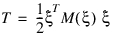 | (59) |
For clarity of presentation we partition the mass matrix,  , into a
  block matrix:
, into a block matrix: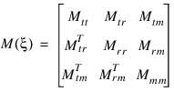 | (60) |
where the subscripts  denote translational, rotational, and modal DOF respectively.
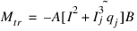
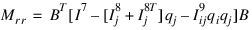
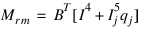
denote translational, rotational, and modal DOF respectively.The expression for the mass matrix  simplifies to an expression in nine inertia invariants.
simplifies to an expression in nine inertia invariants. | (61) |
 | (62) |
 | (63) |
 | (64) |
 | (65) |
 | (66) |
The explicit dependence of the mass matrix on the modal coordinates is evident. The dependence on orientation coordinates of the system comes about because of the transformation matrices  and
and  .
.
and .The inertia invariants are computed from the  nodes of the finite element model based on information about each node’s mass,
  , its undeformed location
  , and its participation in the component modes
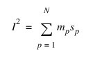
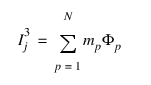
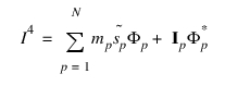
  . The discrete form of the inertia invariants are provided in Table 1.
nodes of the finite element model based on information about each node’s mass, , its undeformed location , and its participation in the component modes . The discrete form of the inertia invariants are provided in Table 1.Table 1 Discrete form of inertia invariants
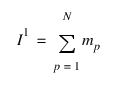 | (scalar) | |
 |  | |
 |  |  |
 |  | |
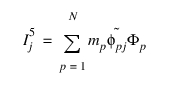 |  |  |
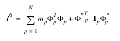 |  | |
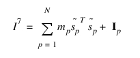 |  | |
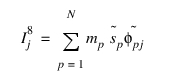 |  |  |
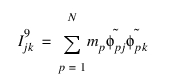 |  |  |
Note: | phi-p-j is mode shape vector {x, y, z} of node p of mode j, and tilde-phipj is skew matrix (3 X 3). |
Potential Energy and the Stiffness Matrix
Frequently, the potential energy consists of contributions from gravity and elasticity in the quadratic form:
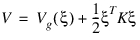 | (67) |
In the elastic energy term,  is the generalized stiffness matrix which is, in general, constant. Only the modal coordinates,
  , contribute to the elastic energy. Therefore, the form of
  is:
is:
is the generalized stiffness matrix which is, in general, constant. Only the modal coordinates, , contribute to the elastic energy. Therefore, the form of is: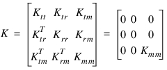 | (68) |
where  is the generalized stiffness matrix of the structural component with respect to the modal coordinates,
  . It is not the full structural stiffness matrix of the component.
is the generalized stiffness matrix of the structural component with respect to the modal coordinates, . It is not the full structural stiffness matrix of the component. is the gravitational potential energy:
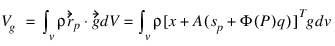 | (69) |
where  denotes the gravitational acceleration vector. The resulting gravitational force,
  is:
is:
denotes the gravitational acceleration vector. The resulting gravitational force, is: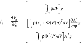 | (70) |
Dissipation and the Damping Matrix
The damping forces depend on the generalized modal velocities and are assumed to be derivable from the quadratic form:
 | (71) |
which is known as Rayleigh’s dissipation function. The matrix  contains the damping coefficients,
  , and is generally constant and symmetric.
contains the damping coefficients, , and is generally constant and symmetric. In the case of orthogonal mode shapes, the damping matrix can be effectively defined using a diagonal matrix of modal damping ratios,  . This damping ratio could be different for each of the orthogonal modes and can be conveniently defined as a ratio of the critical damping for the mode,
  . Recall that the critical damping ratio is defined as the level of damping that eliminates harmonic response as seen in the following derivation. Consider the simple harmonic oscillator defined by uncoupled mode
  .
.
. This damping ratio could be different for each of the orthogonal modes and can be conveniently defined as a ratio of the critical damping for the mode, . Recall that the critical damping ratio is defined as the level of damping that eliminates harmonic response as seen in the following derivation. Consider the simple harmonic oscillator defined by uncoupled mode .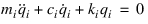 | (72) |
where  denote, respectively, the generalized mass, the generalized stiffness, and the modal damping corresponding to mode
  . Assuming the solution
  , leads to a characteristic equation:
denote, respectively, the generalized mass, the generalized stiffness, and the modal damping corresponding to mode . Assuming the solution , leads to a characteristic equation: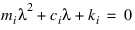 | (73) |
which has the solution:
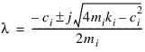 | (74) |
The critical damping of mode  , is the one that eliminates the imaginary part of
  :
:
, is the one that eliminates the imaginary part of : | (75) |
Defining  as a ratio of critical damping introduces the modal damping ratio,
  , which is referred to as CRATIO in the Adams dataset:
as a ratio of critical damping introduces the modal damping ratio, , which is referred to as CRATIO in the Adams dataset: | (76) |
The solution to Equation (72) is:
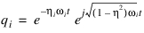 | (77) |
where  is the natural frequency of the undamped system. This solution ceases to be harmonic when
  , which corresponds to 100% of critical damping
is the natural frequency of the undamped system. This solution ceases to be harmonic when , which corresponds to 100% of critical dampingConstraints
Adams satisfies position and orientation constraints for flexible body markers by using the marker kinematics properties presented in Flexible Marker Kinematics. A more complete presentation of Adams joints is beyond the scope of this article.
Governing Differential Equation of Motion--Final Form
The final form of the governing differential equation of motion, in terms of the generalized coordinates is
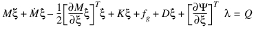 | (78) |
The entries in Equation (78) are:
 | = | the flexible body generalized coordinates and their time derivatives. |
 | = | the flexible body mass matrix in Equation (60). |
 | = | the time derivative of the flexible body mass matrix. |
 | = | the partial derivative of the mass matrix with respect to the flexible body generalized coordinates. This is a  tensor, where tensor, where  is the number of modes. is the number of modes. |
 | = | the generalized stiffness matrix. |
 | = | the generalized gravitational force. |
 | = | the modal damping matrix. |
 | = | the algebraic constraint equations. |
 | = | Lagrange multipliers for the constraints. |
 | = | generalized applied forces. |
Dynamic Limit
Dynamic limit is a feature in Adams Solver (C++) to simplify the equations of motion of high frequency modes by ignoring the inertia terms while keeping the stiffness terms. This will potentially reduce the simulation time, when a significant number of high frequency modes are participating in the solution. Please refer to the DYNAMIC_LIMIT and STABILITY_FACTOR arguments of FLEX_BODY statement in Adams Solver (C++) documentation for detailed information on this feature.