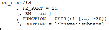
FEloadsub
The FEloadsub evaluation subroutine computes a set of three distributed forces per unit length and three distributed torques per unit length acting on a 3D beam modelled with a FE_PART. The six distributed loads per unit length are named Fx, Fy, Fz, Tx, Ty and Tz. These values are relative to the RM Marker in the FE_LOAD statement. The Fx, Fy, Fz, Tx, Ty and Tz components act relative to the optional RM Marker. If no RM Marker is specified, they are relative to the GROUND origin.
For the case of 2D beam modelled with a FE_PART, the FEloadsub only supports the Fx and Fy distributed force per unit length. Here Fx and Fy are the distributed force per length acting along the XY axes for 2DBEAMXY type. For the case of 2DBEAMYZ, Fx and Fy correspond to the loading along the Y and Z axes respectively. For the case of 2DBEAMZX, Fx and Fy correspond to the loading along the Z and X axes respectively.
You only need to use a FEloadsub if you don't want to use function expressions in the FE_LOAD statement. You may use a FEloadsub when the functions describing the applied distributed loads are too complex to enter as expressions in a FE_LOAD statement.
Specifications
1. Users need to define only one FE_LOAD per FE_PART, regardless of the element subdivision. Changing the number of elements in the FE_PART usually requires no changes in the corresponding FE_LOAD statement. The FE_LOAD expressions (or the FEloadsub code) treat the FE_PART as a single object and apply the load across element boundaries regardless of the element subdivision.
Both FE_PART and FE_LOAD are supported by the Adams/Solver C++ only.
2. The FEloadsub subroutine can only be written in C/C++ code. A FORTRAN version is not supported. To compile a FEloadsub subroutine, follow the standard process used to compile any other supported user-written subroutine.
Important new conventions
To improve the performance of this new type of user-written subroutine, important new conventions were designed and implemented:
1. No numerical perturbation is performed in order to compute the required partial derivatives that Adams Solver C++ needs to carry the simulation. In that regard, the user must provide the partial derivatives when DFLAG=1. To facilitate this task, Adams Solver C++ will call the subroutine passing a data structure named sBeam that can be filled with the corresponding partial derivatives.
2. When IFLAG=1, users must make a call to a new utility function c_sysfn2() for each of the measures needed to compute the distributed loads. Function c_sysfn2() was implemented to register the dependencies.
a. Each call to c_sysfn2() will register a measure and it will return an index for the registered measure.
b. No calls to c_sysfn2() are permitted when IFLAG is different than 1. Adams Solver C++ will compute the values of the registered measures and pass them to your subroutine inside a data structure (see Calling Sequence below).
c. No calls to c_sysfnc() nor c_sysary() are permitted.
For example, assume your distributed loads depend on the following three measures: DX(2), S and SD(1). Assume also you make the following calls in this order:
// Make these calls only when IFLAG=1 (initialization and measure registration)
c_sysfn2( sBeam, "DX", PAR, NPAR, &index, &ERRFLG);
…
c_sysfn2( sBeam, "S", PAR, NPAR, &index, &ERRFLG);
…
c_sysfn2( sBeam, "SD", PAR, NPAR, &index, &ERRFLG);
The index for the measures DX, S and SD will be 0, 1 and 2 respectively, Adams Solver C++ keeps an internal counter. The data structure sBeam is passed to you when Adams Solver C++ calls your subroutine.
3. When IFLAG=3, users must return a map of dependencies for each component. For example, assume your Fx and Fy components have the following expressions:
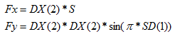
Therefore, when IFLAG=3, you must make the following assignments:
// Make these calls only when IFLAG=3 (mapping of Jacobian dependencies)
sBeam->depend_Fx[0] = 1;
sBeam->depend_Fx[1] = 1;
…
sBeam->depend_Fy[0] = 1;
sBeam->depend_Fy[2] = 1;
…
These settings tell Adams Solver C++ that Fx depends only on the DX measure (index 0) and on the S measure (index 1); similarly this code tells that Fy depends only on the DX measure (index 0) and on the SD measure (index 2).
4. When IFLAG=0, users must return the computed values of the six distributed values Fx, Fy, Fz, Tx, Ty and Tz in the RESULT array. RESULT[0] corresponds to Fx, RESULT[1] corresponds to Fy and so on. Adams Solver C++ will pass the values of all registered measures already computed for you (no need to make calls to c_sysfn2() anymore). The values of the computed measures are passed in the array sBeam->mea_values. For the example above you would do:
// Make this calls only when IFLAG=0 (evaluation)
RESULT[0] = sBeam->mea_values[0]*sBeam->mea_values[1];
RESULT[1] = sBeam->mea_values[0]*sBeam->mea_values[0]*sin(PI*sBeam->mea_values[2]);
…
5. When DFLAG=1, users must return the partial derivatives of each distributed load. Continuing the example above, the corresponding partial derivatives are:
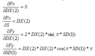
Therefore, the user must code the following:
// Make this calls only when DFLAG=1
sBeam->depend_Fx[0] = sBeam->mea_values[1];
sBeam->depend_Fx[1] = sBeam->mea_values[0];
…
sBeam->depend_Fy[0] = 2.*sBeam->mea_values[0]*sin(PI*sBeam->mea_values[2]);
sBeam->depend_Fy[2] = sBeam->mea_values[0]*sBeam->mea_values[0]*cos(PI*sBeam->mea_values[2])*PI;
…
6. The subroutine FEloadsub can be written in either C or C++. However, if using C++ the subroutine header must be qualified with a leading extern "C" specification. See examples below.
Theoretical background
See documentation on the FE_LOAD for a theoretical background on how the distributed loads are computed and processed by Adams Solver C++.
Use Corresponding Statement
Calling Sequence
If using C:
void FEloadsub( struct sAdamsANCF3DBeamDistrForce *sBeam, double TIME, int DFLAG, int IFLAG, double *RESULT )
If using C++:
extern "C"
void FEloadsub( struct sAdamsANCF3DBeamDistrForce *sBeam, double TIME, int DFLAG, int IFLAG, double *RESULT )
The sAdamsANCF3DbeamDistrForce data structure has the following data members:
struct sAdamsANCF3DBeamDistrForce
{
int ID;
int NPAR;
const double* PAR;
double curr_S;
double *mea_values;
double* depend_Fx;
double* depend_Fy;
double* depend_Fz;
double* depend_Tx;
double* depend_Ty;
double* depend_Tz;
// More data not shown
}
This data structure is passed to the user at every call with the corresponding values of all registered measures (mea_values), the Adams ID of the corresponding FE_LOAD statement (ID), the number of parameters in the USER option (NPAR), the values of all parameters (PAR), the current value of the S location (0<S<1) where the subroutine is being evaluated (curr_S). The other data members are used to pass dependencies and partial derivatives. All of these data members can be accessed in your subroutine code.
Input arguments
sBeam | A pointer to a C++ structure with information about the FE_PART this load is acting upon. File slv_c_utils.h provided more for information about the definition of this data structure. The internal data of this struct is managed entirely by Adams Solver C++. This pointer can be used to (a) retrieve the ID of the FE_PART; (b) find the parameters defined in the USER option of the FE_LOAD statement; (c) register dependencies; (d) get the values of the registered measures; (e) map dependencies. |
TIME | A double-precision variable containing the current simulation time. This variable should be ignored except when IFLAG is 0 or DFLAG is 1. |
DFLAG | An integer variable that Adams Solver C++ sets to 1 when the partial derivatives of the six expressions are requested. Structure sBeam provides the tools to pass the partial derivatives. |
IFLAG | An integer variable that Adams Solver C++ sets to indicate why the routine is being called. 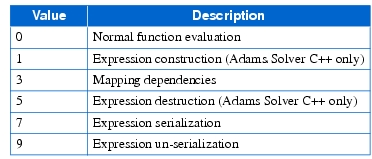 When IFLAG is 1 (expression construction) the user must use the sBeam pointer to "register" the measures the distributed load depends on. Each registration is made by making a call to function c_sysfn2(). Each registered measures is assigned a 0-based index. If the x component of the force depends on 3 measures, the z component of torque depends on 2 components, while the other 4 components of the distributed load are zero, then the user need to register a total of 5 measures. If two or more components depend on the same measure, the measure needs to be registered only once. When IFLG is 3 (expression mapping), the user must provide a map of the partial derivatives of the components relative to the registered measures. If one component of the distributed load (say the x component) depend on the second, fourth and fifth registered measures, then the user should set to 1 the values of the second, fourth and fifth entries of an array provided by the sBeam pointer. When IFLAG is equal to 0, the user should return the value of the distributed force per unit length in array RESULT. Adams Solver C++ passes the values of all registered measures, there is no need to call functions to evaluate the measures. All registered measures can be retrieved from the sBeam pointer. |
Output arguments
RESULT | A double precision array that returns the six values of the distributed force. This array is used only if IFLAG is equal to 0. |
sBeam | Depending on the values of IFLAG and DFLAG, this data structure needs to include additional data explained above. |
Extended Definition
The FE_LOAD statement version using explicit expression is usually adequate for defining functions that represent the three distributed forces per unit length and three distributed torque per unit length. However, if the force and torque expressions are lengthy or complicated, you can use a FEloadsub.
The FEloadsub user-written subroutine requires the user to provide the partial derivatives of the loading with respect to the registered measures. However, in case the loading is complex or no explicit partial derivative expression exists, you may use your own numerical perturbation to approximate the required partial derivatives. See Example 3 and Example 4 below for details.
Example 1
Figure 5 below shows a simple cantilever beam with a sinusoidal distributed loading. The beam has an undeformed length L equal to 6 meters. The left end of the beam is located on the GROUND origin.
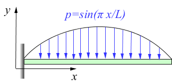
Figure 5 Simple sinusoidal distributed loading.
This loading can be easily defined using a function expression as follows:
FE_LOAD/1
, FE_PART=3
, FX= 0\
, FY= -SIN(PI * SD(1) / 6) \
, FZ= 0\
, TX= 0\
, TY= 0\
, TZ= 0
Function SD(1) returns the value of the x coordinate (in global frame) of the point along the beam where the loading function is evaluated. An equivalent user-written subroutine for this loading would be as follows:
#include "slv_c_utils.h"
#include <math.h>
extern "C"
void FEloadsub( struct sAdamsANCF3DBeamDistrForce* sBeam, double TIME, int DFLAG, int IFLAG, double *RESULT )
{
const double PI = 3.14159265358979323846;
if( IFLAG==1 )
{
int index, ERRFLG, NPAR, PAR[1];
// Registration of measures used by this subroutine
NPAR = 1;
PAR[0] = 1;
c_sysfn2( sBeam, "SD", PAR, NPAR, &index, &ERRFLG );
}
else if( IFLAG==3 )
{
// Mapping dependencies
sBeam->depend_Fy[0] = 1.0;
}
else if( IFLAG==0 )
{
// Normal function evaluation
RESULT[1] = - sin( PI * sBeam->mea_values[0] / 6 );
if( DFLAG==1 )
{
// Returning partial derivatives
sBeam->depend_Fy[0] = - PI * cos( PI * sBeam->mea_values[0] / 6 )/6;
}
}
}
When IFLAG=1 we make the call to c_sysfn2() registering the measure SD(1). When IFLAG=3 we tell Adams Solver the component FY of the loading depends on the SD(1) measure (the index of the SD(1) measure is zero). When IFLAG=0 we return the value for FY. Notice the value of the SD(1) measure is already pre-computed by Adams Solver C++ and passed to the subroutine inside the sBeam->mea_values array. When DFLAG=1 we return the value of the partial derivative of FY with respect to SD(1); notice we use the sBeam->depend_Fy array in order to do so.
Example 2
Given the FE_LOAD statement below, we show a user-written subroutine to perform the computation.
FE_LOAD/1
, FE_PART=3
, FX= COS(SV(3))*SD(2)\
, FY= 2.*SD(1)\
, FZ= 0\
, TX= SD(1)*COS(SD(2))\
, TY= 0\
, TZ= DX(4)*DY(4)
Notice the six components of the FE_LOAD depend on a total of 5 measures: SD(1), SD(2), SV(3), DX(4) and DY(4). Hence, an equivalent subroutine must have a "registration" code as follows:
if( IFLAG==1 )
{
// Registration of measures used by this subroutine
int index;
int ERRFLG;
int PAR[1];
PAR[0] = 1;
c_sysfn2( sBeam, "SD", PAR, 1, &index, &ERRFLG ); // SD(1)
PAR[0] = 2;
c_sysfn2( sBeam, "SD", PAR, 1, &index, &ERRFLG ); // SD(2)
PAR[0] = 3;
c_sysfn2( sBeam, "SV", PAR, 1, &index, &ERRFLG ); // SV(3)
PAR[0] = 4;
c_sysfn2( sBeam, "DX", PAR, 1, &index, &ERRFLG ); // DX(4)
c_sysfn2( sBeam, "DY", PAR, 1, &index, &ERRFLG ); // DY(4)
return;
}
Notice the index variable is not used by the user who wrote this subroutine. If you check the return value of variable index you will notice that measure SD(1) will get a value 0 for the index, SD(2) will get a 1, and so forth. Similarly, for clarity, the ERRFLG is not checked for errors coming from the solver.
During the mapping process (IFLAG=3), the user needs to tell Adams Solver C++ what are the dependencies of each component with respect to the registered measures. For example, if the Fx component depends on measures with index 1 and 2, then the user must set the value 1.0 on the corresponding values in the sBeam data structure. For this example, the registration code would be as follows:
if( IFLAG==3 )
{
// Mapping dependencies
sBeam->depend_Fx[1] = 1.0; // Fx depends on SD(2)
sBeam->depend_Fx[2] = 1.0; // Fx depends on SV(3)
sBeam->depend_Fy[0] = 1.0; // Fy depends on SD(1)
sBeam->depend_Tx[0] = 1.0; // Tx depends on SD(1)
sBeam->depend_Tx[1] = 1.0; // Tx depends on SD(2)
sBeam->depend_Tz[3] = 1.0; // Tz depends on DX(4)
sBeam->depend_Tz[4] = 1.0; // Tz depends on DY(4)
return;
}
Notice arrays depend_FX, depend_FY, depend_FZ, depend_TX, depend_TY and depend_TZ are used to set the dependencies. All entries of those arrays are set to zero before calling the subroutine. Upon returning from the subroutine, Adams Solver C++ will remember those dependencies and expects the partial derivatives are returned on the very same locations when DFLAG is equal to 1.
During normal evaluations (IFLAG equal to 0) the corresponding code should be:
if (IFLAG == 0)
{
// Normal function evaluation
// Fx=cos(SV(3))*SD(2)
RESULT[0] = cos(sBeam->mea_values[2])*(sBeam->mea_values[1]);
// Fy=2*SD(1)
RESULT[1] = 2.0*(sBeam->mea_values[0]);
// Tx=SD(1)*cos(SD(2))
RESULT[3] = (sBeam->mea_values[0])*cos(sBeam->mea_values[1]);
// Tz=DX(4)*DY(4)
RESULT[5] = (sBeam->mea_values[3])*(sBeam->mea_values[4]);
return;
}
Notice the mea_values array returns the values of all the "registered" measures.
During partial derivatives calculations (DFLAG equal to 1) the required partial derivatives can be computed using the mea_values array. The complete example code is as follow:
#include "slv_c_utils.h"
extern "C"
void ANCFbeamsub_two( struct sAdamsANCF3DBeamDistrForce* sBeam, double TIME, int DFLAG, int IFLAG, double *RESULT )
{
if( IFLAG==1 )
{
// Registration of measures used by this subroutine
int index;
int ERRFLG;
int PAR[1];
PAR[0] = 1;
c_sysfn2( sBeam, "SD", PAR, 1, &index, &ERRFLG ); // SD(1)
PAR[0] = 2;
c_sysfn2( sBeam, "SD", PAR, 1, &index, &ERRFLG ); // SD(2)
PAR[0] = 3;
c_sysfn2( sBeam, "SV", PAR, 1, &index, &ERRFLG ); // SV(3)
PAR[0] = 4;
c_sysfn2( sBeam, "DX", PAR, 1, &index, &ERRFLG ); // DX(4)
c_sysfn2( sBeam, "DY", PAR, 1, &index, &ERRFLG ); // DY(4)
return;
}
if( IFLAG==3 )
{
// Mapping dependencies
sBeam->depend_Fx[1] = 1.0;
sBeam->depend_Fx[2] = 1.0;
sBeam->depend_Fy[0] = 1.0;
sBeam->depend_Tx[0] = 1.0;
sBeam->depend_Tx[1] = 1.0;
sBeam->depend_Tz[3] = 1.0;
sBeam->depend_Tz[4] = 1.0;
return;
}
if (IFLAG == 0)
{
// Normal function evaluation
// Fx=cos(SV(3))*SD(2)
RESULT[0] = cos(sBeam->mea_values[2])*(sBeam->mea_values[1]);
// Fy=2*SD(1)
RESULT[1] = 2.0*(sBeam->mea_values[0]);
// Tx=SD(1)*cos(SD(2))
RESULT[3] = (sBeam->mea_values[0])*cos(sBeam->mea_values[1]);
// Tz=DX(4)*DY(4)
RESULT[5] = (sBeam->mea_values[3])*(sBeam->mea_values[4]);
return;
}
if( DFLAG==1 )
{
// Returning partial derivatives
sBeam->depend_Fx[1] = cos(sBeam->mea_values[2]);
sBeam->depend_Fx[2] = -sin(sBeam->mea_values[2])*(sBeam-> mea_values[1]);
sBeam->depend_Fy[0] = 2.0;
sBeam->depend_Tx[0] = cos(sBeam->mea_values[1]);
sBeam->depend_Tx[1] = -sBeam->mea_values[0]*sin(sBeam-> mea_values[1]);
sBeam->depend_Tz[3] = sBeam->mea_values[4];
sBeam->depend_Tz[4] = sBeam->mea_values[3];
return;
}
}
Example 3
Figure 6 below shows a slender cantilever column subject to distributed load due to wind pressure.
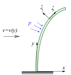
Figure 6 Slender cantilever column.
The distributed load on a beam is specified using components FX, FY, FZ, TX, TY and TZ relative to either GROUND or an RM Marker specified in the FE_LOAD statement. However, in this example we show how we can apply a distributed load normal to the current configuration of the beam.
Let's assume the velocity field and the normal pressure have the following expression:

Hence the pressure to apply is:

The pressure p depends on the value of the y coordinate which is returned by the SD(2) measure. You also need the Euler angles corresponding to the beam's deformed configuration at the point where the distributed force is evaluated (see the local frame x'y' in Figure 6). The Euler 3-1-3 angles of that frame are returned by the SD(4), SD(5) and SD(6) which correspond to the  ,
,  and
and  respectively. With the values of the Euler angles, the instantaneous rotation matrix A has the following expression:
, and respectively. With the values of the Euler angles, the instantaneous rotation matrix A has the following expression: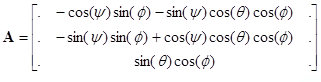
For clarity only the entries corresponding to the local y' axis are shown (center column). The first and third columns define the orientation of the local x' and z' axes respectively. However, those components are no needed in this example. A local pressure p acting in the negative direction y' has the following components in the global reference frame:
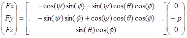
Hence, ignoring the Fz component (assuming the column does not twist), the distributed load has the following expression:
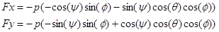
Or
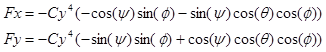
Assume parameter C has a value 0.2 specified in the FE_LOAD statement as follows:
FE_LOAD/7
, FE_PART = 1
, FUNCTION = USER(0.2)
Then the corresponding FEloadsub code for this loading is the following (no RM Marker implies loading is parallel to global origin):
#include "slv_c_utils.h"
#include <math.h>
extern "C"
void FEloadsub( struct sAdamsANCF3DBeamDistrForce* sBeam, double TIME, int DFLAG, int IFLAG, double *RESULT )
{
const double PI = 3.14159265358979323846;
if( IFLAG==1 )
{
// Initialization. Registration of measures used by this subroutine
int index, errflg, npar, par[3];
npar = 1;
par[0] = 2;
c_sysfn2( sBeam, "SD", par, npar, &index, &errflg ); // SD(2) - y position
par[0] = 4;
c_sysfn2( sBeam, "SD", par, npar, &index, &errflg ); // SD(4) - Psi
par[0] = 5;
c_sysfn2( sBeam, "SD", par, npar, &index, &errflg ); // SD(5) - Theta
par[0] = 6;
c_sysfn2( sBeam, "SD", par, npar, &index, &errflg ); // SD(6) - Phi
}
else if( IFLAG==3 )
{
// Mapping dependencies
sBeam->depend_Fx[0] = 1.0;
sBeam->depend_Fx[1] = 1.0;
sBeam->depend_Fx[2] = 1.0;
sBeam->depend_Fx[3] = 1.0;
sBeam->depend_Fy[0] = 1.0;
sBeam->depend_Fy[1] = 1.0;
sBeam->depend_Fy[2] = 1.0;
sBeam->depend_Fy[3] = 1.0;
}
else if( IFLAG==0 )
{
// Normal function evaluation. Get values of parameters and measures
double C = sBeam->PAR[0];
double y = sBeam->mea_values[0];
double Psi = sBeam->mea_values[1];
double Theta = sBeam->mea_values[2];
double Phi = sBeam->mea_values[3];
// Compute the pressure
RESULT[0] = -C*pow(y,4)*(-cos(Psi)*sin(Phi) - sin(Psi)*cos(Theta)*cos(Phi));
RESULT[1] = -C*pow(y,4)*(-sin(Psi)*sin(Phi) + cos(Psi)*cos(Theta)*cos(Phi));
// Partial derivatives
if( DFLAG==1 )
{
sBeam->depend_Fx[0] = -C*4.*pow(y,3)*(-cos(Psi)*sin(Phi) - sin(Psi)*cos(Theta)*cos(Phi));
sBeam->depend_Fx[1] = -C*pow(y,4)*(sin(Psi)*sin(Phi) - cos(Psi)*cos(Theta)*cos(Phi));
sBeam->depend_Fx[2] = -C*pow(y,4)*(sin(Psi)*sin(Theta)*cos(Phi));
sBeam->depend_Fx[3] = -C*pow(y,4)*(-cos(Psi)*cos(Phi) + sin(Psi)*cos(Theta)*sin(Phi));
sBeam->depend_Fy[0] = -C*4.*pow(y,3)*(-sin(Psi)*sin(Phi) + cos(Psi)*cos(Theta)*cos(Phi));
sBeam->depend_Fy[1] = -C*pow(y,4)*(-cos(Psi)*sin(Phi) - sin(Psi)*cos(Theta)*cos(Phi));
sBeam->depend_Fy[2] = -C*pow(y,4)*(-cos(Psi)*sin(Theta)*cos(Phi));
sBeam->depend_Fy[3] = -C*pow(y,4)*(-sin(Psi)*cos(Phi) - cos(Psi)*cos(Theta)*sin(Phi));
}
}
}
Notice the computation of the partial derivatives. Next example discusses the case when the computation of the partial derivatives is done using a simple forward numerical perturbation.
Example 4
This example is based on the previous example. The computation of the required partial derivatives may be time consuming or difficult in some cases. In that regard, you may compute the partial derivatives doing your own numerical perturbation as the following code shows. For example, you could write the following functions to compute Fx and Fy (compare with Example 3 above):
double myFx( double C, double y, double Psi, double Theta, double Phi )
{
return -C*pow(y,4)*(-cos(Psi)*sin(Phi) - sin(Psi)*cos(Theta)*cos(Phi));
}
double myFy( double C, double y, double Psi, double Theta, double Phi )
{
return -C*pow(y,4)*(-sin(Psi)*sin(Phi) + cos(Psi)*cos(Theta)*cos(Phi));
}
Also, a perturbation parameter H is defined with the value 0.0001. The user-written subroutine can now be written as follows:
extern "C"
void FEloadsub( struct sAdamsANCF3DBeamDistrForce* sBeam, double TIME, int DFLAG, int IFLAG, double *RESULT )
{
const double PI = 3.14159265358979323846;
const double H = 0.0001;
if( IFLAG==1 )
{
// Initialization. Registration of measures used by this subroutine
int index, errflg, npar, par[3];
npar = 1;
par[0] = 2;
c_sysfn2( sBeam, "SD", par, npar, &index, &errflg ); // SD(2) - y position
par[0] = 4;
c_sysfn2( sBeam, "SD", par, npar, &index, &errflg ); // SD(4) - Psi
par[0] = 5;
c_sysfn2( sBeam, "SD", par, npar, &index, &errflg ); // SD(5) - Theta
par[0] = 6;
c_sysfn2( sBeam, "SD", par, npar, &index, &errflg ); // SD(6) - Phi
}
else if( IFLAG==3 )
{
// Mapping dependencies
sBeam->depend_Fx[0] = 1.0;
sBeam->depend_Fx[1] = 1.0;
sBeam->depend_Fx[2] = 1.0;
sBeam->depend_Fx[3] = 1.0;
sBeam->depend_Fy[0] = 1.0;
sBeam->depend_Fy[1] = 1.0;
sBeam->depend_Fy[2] = 1.0;
sBeam->depend_Fy[3] = 1.0;
}
else if( IFLAG==0 )
{
// Normal function evaluation. Get values of parameters and measures
double C = sBeam->PAR[0];
double y = sBeam->mea_values[0];
double Psi = sBeam->mea_values[1];
double Theta = sBeam->mea_values[2];
double Phi = sBeam->mea_values[3];
// Compute the pressure
RESULT[0] = myFx( C, y, Psi, Theta, Phi );
RESULT[1] = myFy( C, y, Psi, Theta, Phi );
// Partial derivatives computed numerically
if( DFLAG==1 )
{
sBeam->depend_Fx[0] = (myFx(C, y+H, Psi, Theta, Phi)-myFx(C, y, Psi, Theta, Phi))/H;
sBeam->depend_Fx[1] = (myFx(C, y, Psi+H, Theta, Phi)-myFx(C, y, Psi, Theta, Phi))/H;
sBeam->depend_Fx[2] = (myFx(C, y, Psi, Theta+H, Phi)-myFx(C, y, Psi, Theta, Phi))/H;
sBeam->depend_Fx[3] = (myFx(C, y, Psi, Theta, Phi+H)-myFx(C, y, Psi, Theta, Phi))/H;
sBeam->depend_Fy[0] = (myFy(C, y+H, Psi, Theta, Phi)-myFy(C, y, Psi, Theta, Phi))/H;
sBeam->depend_Fy[1] = (myFy(C, y, Psi+H, Theta, Phi)-myFy(C, y, Psi, Theta, Phi))/H;
sBeam->depend_Fy[2] = (myFy(C, y, Psi, Theta+H, Phi)-myFy(C, y, Psi, Theta, Phi))/H;
sBeam->depend_Fy[3] = (myFy(C, y, Psi, Theta, Phi+H)-myFy(C, y, Psi, Theta, Phi))/H;
}
}
}
The computation of the partial derivatives does not need to be exact. Adams Solver C++ uses a Newton-Raphson algorithm to solve the nonlinear governing equations. In that regard, the partial derivatives provided to the Solver may be simplified. In some case you may choose to ignore computing partial derivatives.