BEAM
The BEAM statement defines a force and a torque corresponding to a massless elastic beam with a uniform cross section. The beam transmits forces and torques between two markers in accordance with either linear Timoshenko beam theory or the non-linear Euler-Bernoulli theory. Conversely to standard Finite Elements codes, the BEAM element defines a force-only element; no equations of motion for the mass of the beam are formulated.
The BEAM statement supports three formulations to construct the force and torque expressions for this element. By default, the linear Timoshenko beam theory is used (see Using the FORMULATION=LINEAR option below); this default model is the one used in previous versions of Adams Solver C++. However, the FORMULATION option is available in order to use either a full non linear Euler-Bernoulli theory or a simplified non linear theory.
Format
Arguments
AREA=r | Specifies the uniform area of the beam cross section. The centroidal axis must be orthogonal to this cross section. |
ASY=r | Specifies the correction factor (that is, the shear area ratio) for shear deflection in the y direction for Timoshenko beams. 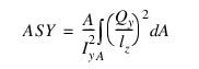 where Qy is the first moment of cross-sectional area to be sheared by a force in the z direction, and Iz is the cross section dimension in the z direction. If you want to neglect the deflection due to y-direction shear, ASY does not need to be included in a BEAM statement. Defaults: 0 |
ASZ=r | Specifies the correction factor (that is, the shear area ratio) for shear deflection in the z direction for Timoshenko beams. 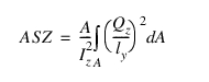 where Qz is the first moment of cross-sectional area to be sheared by a force in the y direction, and Iy is the cross section dimension in the y direction. If you want to neglect the deflection due to z-direction shear, ASZ does not need to be included in a BEAM statement. Defaults: 0 Commonly encountered values for the shear area ratio are: 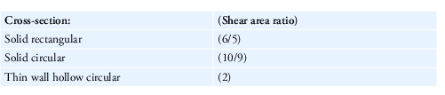 See also “Roark’s Formulas for Stress and Strain,” Young, Warren C., Sixth Edition, page 201. New York:McGraw Hill, 1989. |
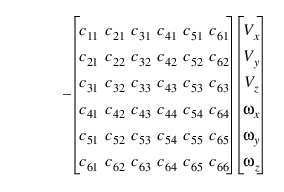
CMATRIX=r1,...,r21 | Establishes a six-by-six damping matrix for the beam. Because this matrix is symmetric, only one-half of it needs to be specified. The following matrix shows the values to input:  Enter the elements by columns from top to bottom, then by rows from left to right. If you do not use either CMATRIX or CRATIO, CMATRIX defaults to a matrix with thirty-six zero entries; that is, r1 through r21 each default to zero. |
CRATIO=r | Establishes a ratio for calculating the damping matrix for the beam. Adams Solver multiplies the stiffness matrix by the value of CRATIO to obtain the damping matrix. Defaults: 0 |
EMODULUS=r | Defines Young’s modulus of elasticity for the beam material. |
GMODULUS=r | Defines the shear modulus of elasticity for the beam material. |
I=id, J=id | Specifies the two markers between which to define a beam. The J marker establishes the direction of the force components. |
IXX=r | Denotes the torsional constant. This is sometimes referred to as the torsional shape factor or torsional stiffness coefficient. It is expressed as unit length to the fourth power. For a solid circular section, Ixx is identical to the polar moment of inertia  where r is the radius of the cross-section. where r is the radius of the cross-section. For thin-walled sections, open sections, and noncircular sections, you should consult a handbook. |
IYY=r,IZZ=r | Denote the area moments of inertia about the neutral axes of the beam cross sectional areas (y-y and z-z). These are sometimes referred to as the second moment of area about a given axis. They are expressed as unit length to the fourth power. For a solid circular section, Iyy=Izz=  where r is the radius of the cross-section. where r is the radius of the cross-section. For thin-walled sections, open sections, and noncircular sections, you should consult a handbook. |
LENGTH=r | Defines the underformed length of the beam along the x-axis of the J marker. |
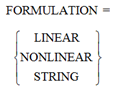 | Specifies the formulation to be used to define the force and torque this element will apply. By default the LINEAR theory is used (see Using the FORMULATION=LINEAR option below). If the NONLINEAR option is used, the full non linear Euler-Bernoulli theory is used. If the STRING option is used, a simplified non linear theory is used. The simplified non linear theory may speed up your simulations with little performance penalties. |
Extended Definition
The figure below shows the two markers (I and J) that define the extremities of the beam and indicates the twelve forces (s1 to s12) it produces.
The x-axis of the J marker defines the centroidal axis of the beam. The y-axis and z-axis of the J marker are the principal axes of the cross section. They are perpendicular to the x-axis and to each other. When the beam is in an undeflected position, the I marker has the same angular orientation as the J marker, and the I marker lies on the x-axis of the J marker a distance LENGTH away.
The beam statement applies the following forces to the I marker in response to the relative motion of the I marker with respect to the J marker (see nomenclature in Figure above):
■Axial forces (s1 and s7)
■Bending moments about the y-axis and z-axis (s5, s6, s11, and s12)
■Twisting moments about the x-axis (s4 and s10)
■Shear forces (s2, s3, s8, and s9)
Using the FORMULATION=LINEAR option
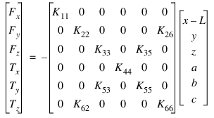
When using the default FORMULATION or when explicitly using FORMULATION=LINEAR, the linear Timoshenko beam theory is used to define the forces and moments. In this case Adams Solver (C++) uses a linear translational and linear rotational action-reaction force between the two markers I and J. The forces the beam produces are linearly dependent on the displacements, rotations, and corresponding velocities between the markers at its endpoints.
The following constitutive equations define how Adams Solver applies a force and a torque to the I marker depending on the displacement rotation and velocity of the I marker relative to the J marker.
where:
■Fx, Fy, and Fz are the measure numbers of the translational force components in the coordinate system of the J marker.
■x, y, and z are the translational displacements of the I marker with respect to the J marker measured in the coordinate system of the J marker.
■Vx, Vy, and Vz are the time derivatives of x, y, and z, respectively.
■Tx, Ty, and Tz are the rotational force components in the coordinate system of the J marker.
■a, b, and c are the relative rotational displacements of the I marker with respect to the J marker as expressed in the x-, y-, and z-axis, respectively, of the J marker.
■ ,
,  , and
, and  are the components of the angular velocity of the I marker with respect to the J marker, as seen by the J marker and measured in the J marker coordinate system.
, , and are the components of the angular velocity of the I marker with respect to the J marker, as seen by the J marker and measured in the J marker coordinate system. ■Cij are the entries of the damping matrix either specified by the CMATRIX option or computed by using the CRATIO option. All Cij entries default to zero.
Note that both matrices, Cij and Kij, are symmetric, that is, Cij=Cji and Kij=Kji. You define the twenty-one unique damping coefficients when the BEAM statement is written. Adams Solver (C++) defines each Kij as follows:
Adams Solver (C++) applies an equilibrating force and torque at the J marker, as defined by the following equations:
Fj = - Fi
Tj = - Ti - L x Fi
Tj = - Ti - L x Fi
L is the instantaneous vector from the J marker to the I marker. While the force at the J marker is equal and opposite to the force at the I marker, the torque is usually not equal and opposite, because of vector L.
The BEAM statement implements a force in the same way the FIELD statement does, but the BEAM statement requires you to input only the values of the beam’s physical properties, which Adams Solver (C++) uses to calculate the matrix entries.
Using the FORMULATION=NONLINEAR option
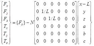
When using the FORMULATION=NONLINEAR option, then the Euler-Bernoulli formulation is used to define the forces and moments. In this case, Adams Solver (C++) uses the following constitutive equations to apply a force and a torque to the I marker.
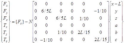
Where  corresponds to the Timoshenko's constitutive equations shown above, and N is the axial force on the beam computed as:
corresponds to the Timoshenko's constitutive equations shown above, and N is the axial force on the beam computed as: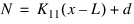
The axial force N corresponds to the term Fx computed using linear theory (see section Using the FORMULATION=LINEAR option above.) If there is damping (options CRATIO or CMATRIX are used), the term d corresponds to viscous damping and can be computed as shown above. See reference [2] for more information.
The linear theory is the default model for the BEAM statement. The non linear theory should be used when the BEAM elements in the model are subject to high axial forces. In those cases, the additional terms in the force/torque equations help stabilize the numerical solution.
Using the FORMULATION=STRING option
When using the option FORMULATION=STRING, then a simplified Euler-Bernoulli formulation is used to define the forces and moments. In this case, Adams Solver (C++) uses the following constitutive equations to apply a force and a torque to the I marker.
Where  and N are computed as described in Using the FORMULATION=NONLINEAR option above. This simplification may provide accurate results faster. See Chapter 15 in reference [2] for more details on string stiffness. Notice the stiffness matrices shown in all of the above equations show only a subset of a complete stiffness matrix displayed in textbooks. The rest of the entries may be found applying equilibrium conditions.
and N are computed as described in Using the FORMULATION=NONLINEAR option above. This simplification may provide accurate results faster. See Chapter 15 in reference [2] for more details on string stiffness. Notice the stiffness matrices shown in all of the above equations show only a subset of a complete stiffness matrix displayed in textbooks. The rest of the entries may be found applying equilibrium conditions.Discussion
The BEAM element is a useful force/torque element but it does include inertial effects. If you need to include inertial effects, see the FE_PART statement.
The fastest simulation time in the majority of cases is provided by the default formulation (FORMULATION=LINEAR). However, the LINEAR formulation may lead into a simulation failure due to instabilities if axial forces are high. The typical case is that of slender blades modelled using PARTs connected by BEAMs and rotating at high angular speed. High axial loads may introduce numerical instabilities. In order to obtain a stable and correct numerical solution, the NONLINEAR formulation is required in those cases. Unfortunately, the NONLINEAR option requires higher simulation time due to the complex expressions for the force and torque. In some cases, using the STRING option may speed up the simulation time while providing accurate results.
Beam Forces
When using the BEAM element, the best idealization of beam flexibility uses the principle of using enough BEAMs to model the desired flexibility. For reasons of practicality, if you model flexibility by only one BEAM, you should keep in mind that the forces on the I and J markers may NOT be transposable. That is, the BEAM forces may not be symmetric when the I and J marker locations are switched. See the last Caution note below for an explanation. The following figures illustrate this asymmetry and how to overcome it.
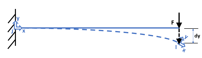
Figure 1 Cantilever Beam with J Marker Grounded
In Figure 1 the J marker of the BEAM is fixed to ground. Since the BEAM uses the J marker as its reference frame, it behaves as a finite element BEAM would, giving non-zero displacement in the Y axis of the J marker and zero displacement along the x axis of the J marker.
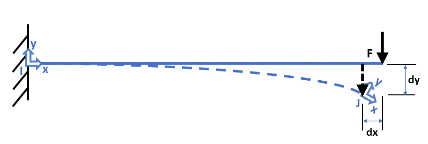
Figure 2 Cantilever Beam with I Marker Grounded
Here, the I and J markers are reversed, and the J marker is no longer constrained to ground. Thus, when the force F causes the beam to deflect and the J marker to rotate, the force is applied along the x and y axis of the J marker – not only along the y axis as was the case in the previous model. The forces resulting from the BEAM depend on the J marker kinematics. As a result, do not expect the BEAM forces on the I and J markers to be the same in each example.
Next is the model of a pinned beam shown in Figure 3 that has Part A attached to ground with a revolute Joint A. Part B is attached to ground with a revolute Joint B. Part A and Part B are connected with a BEAM. While this model may appear symmetrical, it is not by definition, and you will not get symmetric results in the BEAM forces
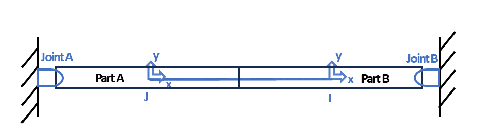
Figure 3 Pinned Beam
Figure 4 shows how this can be avoided by modeling symmetrically by adding a dummy part and more beams.
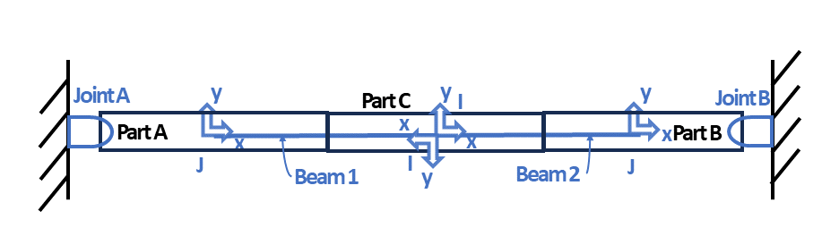
Figure 4 Symmetric Model of a Pinned Beam
The model from Figure 3 has been modified in Figure 4to incl dummy Part C that is connected to Part A and Part B with Beams 1 and Beam 2. As more beams are added, the effect illustrated in Figure 1and Figure 2 are more localized, and the solution becomes less sensitive to the locations of the I and J markers of the BEAM elements
Tip: | ■A FIELD statement can be used instead of a BEAM statement to define a beam with characteristics unlike those the BEAM statement assumes. For example, a FIELD statement should be used to define a beam with a nonuniform cross section or a beam with nonlinear material characteristics. ■The beam element in Adams Solver (C++) is similar to those in most finite element programs. That is, the stiffness matrix that Adams Solver (C++) computes is the standard beam element stiffness matrix. ■The USEXP option on the MARKER statement may make it easier to direct the x-axis of the J marker. ■Generally, it is desirable to define the x-axis of the Adams Solver (C++) beam on the shear center axis of the beam being modeled. |
Caution: | ■The K1 and K2 terms used by MSC.NASTRAN for defining the beam properties using PBEAM are inverse of the ASY and ASZ used by Adams Solver (C++). ■When the x-axes of the markers defining a beam are not collinear, the beam deflection and, consequently, the force corresponding to this deflection are nonzero. To minimize the effect of such misalignments, perform a static equilibrium at the start of the simulation. ■By definition, the beam lies along the positive x-axis of the J marker. (This is unlike most other Adams Solver (C++) force statements, for which the z-axis is the significant axis.) Therefore, the I marker must have a positive x displacement with respect to the J marker when viewed from the J marker. In its undeformed configuration, the orientation of the I and the J markers must be the same. ■The damping matrix that CMATRIX specifies should be positive semidefinite. This ensures that damping does not feed energy into the system. Adams Solver (C++) does not warn you if CMATRIX is not positive semidefinite. ■When the beam element angular deflections are small, the stiffness matrix provides a meaningful description of beam behavior. However, when the angular deflections are large, they are not commutative; so the stiffness matrix that produces the translational and rotational force components may not correctly describe the beam behavior. If BEAM translational displacements exceed ten percent of the undeformed LENGTH, then Adams Solver issues a warning message. ■By its definition a BEAM is asymmetric. Holding the J marker fixed and deflecting the I marker produces different results than holding the I marker fixed and deflecting the J marker by the same amount. This asymmetry occurs because the coordinate system frame that the deflection of the BEAM is measured in moves with the J marker. |
Examples
A cantilevered stainless steel beam is to be modeled with a circular cross section that has the loading shown in the figure below.
A weight of 17.4533 lbf at the free end of the beam with a 100-inch axial offset in the negative y direction causes torsion to the beam as shown in the figure above. The following statement defines this beam:
BEAM/0201, I=0010, J=0020, LENGTH=100
, IXX=100, IYY=50, IZZ=50, AREA=25.0663
, ASY=1.11, ASZ=1.11, EMOD=28E6, GMOD=10.6E6,
, CRATIO=0.0001
, IXX=100, IYY=50, IZZ=50, AREA=25.0663
, ASY=1.11, ASZ=1.11, EMOD=28E6, GMOD=10.6E6,
, CRATIO=0.0001
The beam lies between Marker 0010 and Marker 0020. The length of the beam is 100 inches; its torsional constant is 100 inch4; its principal area moments of inertia about the y-axis is 50 inch4, and about the z-axis is 50 inch4; its cross-sectional area is 25.0663 inch2; its shear area ratio in the y direction is 1.11; its shear area ratio in the z direction is 1.11; its modulus of elasticity is 28E6 psi; its shear modulus is 10.6 psi; and its damping ratio relative to the stiffness matrix Adams Solver (C++) calculates is 0.0001. Note that the beam ends belong to different parts.
References
1. Roark's Formulas for Stress and Strain, Young, Warren C., Sixth Edition, page 201. New York: McGraw Hill, 1989.
2. J.S. Przemieniecki, Theory of Matrix Structural Analysis. New York: McGraw-Hill Book Company, 1968
See other Forces available.