SYSPAR
The SYSPAR subroutine lets you supply the analytical partial derivatives of a subroutine with respect to values measured through SYSFNC and SYSARY.
When you supply analytical partial derivatives, Adams Solver does not need to resort to finite differencing to approximate these partial derivatives. Therefore, you potentially improve both accuracy and speed.
SYSPAR can be used for any number (all, some, or none) of the SYSFNC or SYSARY calls made from your subroutine.
You can also use SYSPAR intermittently. For example, you can use it only during the first half of the simulation. Adams Solver will use the values you provide, when you provide them, and compute them automatically when you do not.
Note: | SYSPAR works primarily in the Adams Solver (C++) or with the GSE statement in Adams Solver FORTRAN. |
Use
Called By
Any user subroutine that can call SYSFNC and SYSARY.
Calling Sequence
CALL SYSPAR (fncname, iparam, nparam, partl, npartl, errflg)
Input Arguments
fncname | A character variable specifying the name of the function corresponding to the partial derivatives that are being provided. The legal values for fncname are derived from the list of functions available to you in the FUNCTION = expression construct. Depending on the subroutine you are calling, see either SYSARY or SYSFNC for a list of legal characters. |
iparam | An integer array containing the parameter list for fncnam. It consists of any valid list of parameters used in the associated Adams Solver function, just as they would appear in a dataset FUNCTION = expression. |
nparam | An integer variable specifying the number of values in ipar. |
partl | Array of partial derivatives that you computed. |
npartl | Number of partial derivatives in partl. Adams Solver compares this number with the number that it expects, and issues an error message if you provide an incorrect number of partial derivatives. |
Output Arguments
errflg | A logical variable that returns true if an error has occurred during your call to SYSPAR. |
Extended Definition
Adams Solver offers a number of user subroutines that you can use to define the value of Adams variables, differential equations, forces, and so on. The subroutines return values of dimension 1, 3, or 6. Usually, the subroutines have a dependency on system states through measurements of the system state provided by a functional interface, SYSFNC and SYSARY. We define the following nomenclature:
F - The value computed by the user subroutine
Mi - The ith measured value
q - The system generalized coordinates
and observe that, in general:
F(M1(q), M2 (q), ..., MN (q))
Because the user subroutine is effectively a closed box, all that Adams Solver knows about this function is that it depends on the measures, Mi, that you call through SYSFNC/SYSARY.
During its analyses, Adams Solver must construct a Jacobian matrix of the system of equations. For this purpose, Adams Solver requires the partial derivatives,  , of the function relative to the system-generalized coordinates, q.
, of the function relative to the system-generalized coordinates, q. The FORTRAN 77 version of Adams Solver approaches the problem of computing these partial derivatives in a direct manner, by altering the system states:
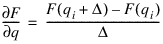
We refer to this scheme as finite differencing or, more specifically, forward differencing. This approach has two main problems:
■Some Adams elements, particularly the FLEX_BODY element, can have an extremely large number of generalized coordinates. Computing the partial derivatives in this way can be quite time consuming. Note that during finite differencing the user subroutine must be evaluated once for each state, qi, on which it depends.
■You cannot assist Adams Solver in the evaluation of the partial derivatives because you do not have direct access to the generalized coordinates, q, that Adams uses.
To address these problems, the C++ version of Adams Solver takes a different approach to computing the partial derivatives. The C++ version applies the chain rule:
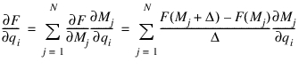
Note that in keeping with the observation that F is a closed box, Adams Solver continues to rely on finite differencing to compute  , where Mj is well known and its partial derivatives can be evaluated analytically. This scheme solves both problems:
, where Mj is well known and its partial derivatives can be evaluated analytically. This scheme solves both problems: ■During finite differencing, the user subroutine only needs to be evaluated as many times as the total dimension of all the measures.
For example, if F depends on the 3D TDISP measure of a marker on a FLEX_BODY, F must only be evaluated three times during finite differencing, even if the FLEX_BODY has 200 modal generalized coordinates. This is a remarkable computational savings.
Note that the computational savings are not always so generous. Consider a function F that depends on the two 6D measures, DISP and VEL, of a single PART marker, with respect to ground. During finite differencing, F must be evaluated 12 times, once for each dimension of each measure. Meanwhile, the function only depends on the 12 generalized displacements and velocities of the PART, so the FORTRAN 77 Adams Solver would also only have needed 12 evaluations of F.
■Because you are aware of the functional dependency of the function, F, on the measured quantities, Mi, computing  may be straightforward. Adams Solver (C++) provides SYSPAR: an interface you can use to register these partial derivatives, in the cases where they are known and can be efficiently computed.
may be straightforward. Adams Solver (C++) provides SYSPAR: an interface you can use to register these partial derivatives, in the cases where they are known and can be efficiently computed. Note that the potential of user-provided partial derivatives does not only affect the computational cost of evaluating the system Jacobian, but can also improve the accuracy of simulations and the rate of convergence. This is because your analytical derivatives are likely to be more accurate than those obtained using finite differencing. When Adams Solver uses the Jacobian directly, as in Adams Linear, the quality of the solution may also be improved.
When F and M have dimension greater than 1, the partial matrix,  should be stored in partl in FORTRAN 77 style column order. In other words, all the partial derivatives of F with respect to the first component of M come before the partial derivatives of F with respect to the second component of M, and so on.
should be stored in partl in FORTRAN 77 style column order. In other words, all the partial derivatives of F with respect to the first component of M come before the partial derivatives of F with respect to the second component of M, and so on. Each call to SYSFNC/SYSARY creates what the previous section refers to as a measure. For each of these measures, the creator of the user subroutine is allowed to register the partials of the function with respect to this measure.
You do not need partial derivatives during every call to the user's subroutine, because they are only needed when the Jacobian is being evaluated. You must request the flag that indicates whether the partial derivatives are required, by calling the following function:
CALL ADAMS_NEEDS_PARTIALS(PARFLG)
Note that, ideally, the PARFLG would have been added to the user subroutine call, alongside IFLAG and DFLAG, but the user subroutines have a standard interface that cannot be changed.
You can make calls to SYSPAR only for those SYSFNC/SYSARY for which partials are conveniently available. As mentioned earlier, you can make SYSPAR calls intermittently. In other words, you can call SYSPAR only during some period of the simulation when partials can be easily computed, but skipped during other parts of the simulation. For example, when an impact force is zero, its partials are trivially zero.
Caution: | SYSPAR is optional. You should expect the number of function evaluations and CPU time to decrease. If they do not, you may have made a mistake. When you do not provide partial information, Adams Solver fills in the blanks using finite differencing. It is, of course, an error to call SYSPAR without a matching call to SYSFNC or SYSARY. |
Examples
Using an SFOSUB with SYSPAR
The following example shows how a SFOSUB has been modified to use SYSPAR. The SFOSUB computes VALUE = DX(1,2)*VZ(1,2).
Relating this to the terminology used earlier, we have:
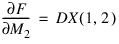
F = M1 M2
where M1 = DX(1,2) and M2 = VZ(1,2). Consequently:
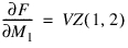
and
The SFOSUB implementation follows:
SUBROUTINE SFOSUB (ID, TIME, PAR, NPAR, DFLAG, IFLAG, VALUE)
INTEGER ID
DOUBLE PRECISION TIME
DOUBLE PRECISION PAR( * )
INTEGER NPAR
LOGICAL DFLAG
INTEGER IFLAG
DOUBLE PRECISION VALUE
DOUBLE PRECISION TIME
DOUBLE PRECISION PAR( * )
INTEGER NPAR
LOGICAL DFLAG
INTEGER IFLAG
DOUBLE PRECISION VALUE
DOUBLE PRECISION DX, VZ
INTEGER NUM, IPAR(2)
LOGICAL ERRFLG
LOGICAL PARFLG
INTEGER NUM, IPAR(2)
LOGICAL ERRFLG
LOGICAL PARFLG
CALL ADAMS_NEEDS_PARTIALS(PARFLG)
IPAR(1) = PAR(1)
IPAR(2) = PAR(2)
IPAR(2) = PAR(2)
CALL SYSFNC('DX', IPAR, 2, DX, ERRFLG )
CALL SYSFNC('VZ', IPAR, 2, VZ, ERRFLG )
VALUE = DX*VZ
CALL SYSFNC('VZ', IPAR, 2, VZ, ERRFLG )
VALUE = DX*VZ
IF(PARFLG) THEN
CALL SYSPAR('DX', IPAR, 2, VZ, 1, ERRFLG)
CALL SYSPAR('VZ', IPAR, 2, DX, 1, ERRFLG)
ENDIF
CALL SYSPAR('DX', IPAR, 2, VZ, 1, ERRFLG)
CALL SYSPAR('VZ', IPAR, 2, DX, 1, ERRFLG)
ENDIF
CALL ERRMES(ERRFLG,'ERROR FOR SFORCE ',ID,'STOP')
RETURN
END
END
Using SYSPAR with Utility Subroutines
This SFOSUB example shows how you can use SYSPAR in conjunction with utility subroutines. In this SFOSUB you have:
VALUE = -IMPACT(400-DM(12,9),-VR(12,9))
or, using the nomenclature developed earlier:
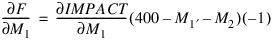
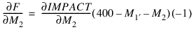
F = -IMPACT(400-M1,-M2)
where M1 = DM(12,9) and M2 = VR(12,9). Here, you must rely on the ability of the IMPACT utility function to provide partial derivatives of its arguments.
The implementation follows. Pay close attention to the use of the IORD argument (argument 8) to the IMPACT function. It controls whether 0th, 1st, or 2nd derivative of the impact is being requested. Learn more about the IMPACT function (C++ or FORTRAN).
SUBROUTINE SFOSUB (ID, TIME, PAR, NPAR, DFLAG, IFLAG, VALUE)
INTEGER ID
DOUBLE PRECISION TIME
DOUBLE PRECISION PAR( * )
INTEGER NPAR
LOGICAL DFLAG
INTEGER IFLAG
DOUBLE PRECISION VALUE
INTEGER ID
DOUBLE PRECISION TIME
DOUBLE PRECISION PAR( * )
INTEGER NPAR
LOGICAL DFLAG
INTEGER IFLAG
DOUBLE PRECISION VALUE
DOUBLE PRECISION DM, VR, V(3)
INTEGER IPAR(2)
LOGICAL ERRFLG, PARFLG
INTEGER IPAR(2)
LOGICAL ERRFLG, PARFLG
IPAR(1)=12
IPAR(2)=9
IPAR(2)=9
CALL ADAMS_NEEDS_PARTIALS(PARFLG)
CALL SYSFNC('DM', IPAR, 2, DM, ERRFLG )
CALL SYSFNC('VR', IPAR, 2, VR, ERRFLG )
CALL SYSFNC('VR', IPAR, 2, VR, ERRFLG )
IF(PARFLG) THEN
CALL IMPACT(400.D0-DM,-VR,100D0,1.D2,1.5D0, 1D1,1.D0,1,V,ERRFLG)
CALL SYSPAR('DM', IPAR, 2, V(1), 1, ERRFLG )
CALL SYSPAR('VR', IPAR, 2, V(2), 1, ERRFLG )
ENDIF
CALL IMPACT(400.D0-DM,-VR,100D0,1.D2,1.5D0, 1D1,1.D0,1,V,ERRFLG)
CALL SYSPAR('DM', IPAR, 2, V(1), 1, ERRFLG )
CALL SYSPAR('VR', IPAR, 2, V(2), 1, ERRFLG )
ENDIF
CALL IMPACT(400-DM,-VR,100D0,100.0D0,1.5D0,10D0,1.0D0,0,V,ERRFLG)
VALUE=-V(1)
VALUE=-V(1)
CALL ERRMES(ERRFLG,'ERROR FOR SFORCE',ID,'STOP')
RETURN
END
END
Using FIESUB with SYSPAR
This example, involving FIESUB, shows how SYSPAR has closed the functionality gap between GFOSUB and FIESUB. In the FORTRAN 77 version of Adams Solver, the ability to define partial derivatives of the FIELD element in a FIESUB user subroutine gives it a computational advantage over the GFORCE force element and a GFOSUB user subroutine. The FIESUB user subroutine is defined as follows:
CALL FIESUB(ID, TIME, PAR, NPAR, DISP, VELO,
DFLAG, IFLAG, FIELD, DFDDIS, DFDVEL)
DFLAG, IFLAG, FIELD, DFDDIS, DFDVEL)
where DISP and VELO are the displacement and velocity of the I and J markers of the field element that are input to FIESUB. FIESUB computes the 6D value of the force, FIELD. Also, when DFLAG is TRUE, you must provide the partial derivatives with respect to displacement, DFDDIS, and the partial derivatives with respect to velocity, DFDVEL. Learn more about FIELD (C++ or FORTRAN).
The removal of the advantage of FIESUB over GFOSUB is demonstrated by implementing the FIESUB in a GFOSUB:
SUBROUTINE GFOSUB (ID, TIME, PAR, NPAR, DFLAG, IFLAG, RESULT)
INTEGER ID
DOUBLE PRECISION TIME
DOUBLE PRECISION PAR( * )
INTEGER NPAR
LOGICAL DFLAG
INTEGER IFLAG
DOUBLE PRECISION RESULT(6)
INTEGER ID
DOUBLE PRECISION TIME
DOUBLE PRECISION PAR( * )
INTEGER NPAR
LOGICAL DFLAG
INTEGER IFLAG
DOUBLE PRECISION RESULT(6)
DOUBLE PRECISION DISP(6), VELO(6)
DOUBLE PRECISION DFDDIS(6,6), DFDVEL(6,6)
DOUBLE PRECISION DFDDIS(6,6), DFDVEL(6,6)
INTEGER IPAR(4)
LOGICAL ERRFLG, PARFLG
C
C This GFOSUB should never be finite differenced
C
CALL ERRMES(DFLAG,'DFLAG=.TRUE. UNEXPECTED',ID,'STOP')
C
C Check if partials are needed
C
CALL ADAMS_NEEDS_PARTIALS(PARFLG)
C
C Measure displacements, projection angles and velocity
C between markers I and J (PAR(1) and PAR(2)). Note that
C velocity measure takes four marker arguments because
C FIESUB uses velocity of I wrt J in coordinate system
C of J with observer in J.
C
IPAR(1)=NINT(PAR(1))
IPAR(2)=NINT(PAR(2))
IPAR(3)=NINT(PAR(2))
IPAR(4)=NINT(PAR(2))
IPAR(2)=NINT(PAR(2))
IPAR(3)=NINT(PAR(2))
IPAR(4)=NINT(PAR(2))
C
CALL SYSARY('TDISP', IPAR, 3, DISP, 3, ERRFLG )
CALL SYSFNC('AX', IPAR, 2, DISP(4), ERRFLG )
CALL SYSFNC('AY', IPAR, 2, DISP(5), ERRFLG )
CALL SYSFNC('AZ', IPAR, 2, DISP(6), ERRFLG )
CALL SYSARY('VEL', IPAR, 4, VELO, 6, ERRFLG )
CALL SYSFNC('AX', IPAR, 2, DISP(4), ERRFLG )
CALL SYSFNC('AY', IPAR, 2, DISP(5), ERRFLG )
CALL SYSFNC('AZ', IPAR, 2, DISP(6), ERRFLG )
CALL SYSARY('VEL', IPAR, 4, VELO, 6, ERRFLG )
IF(PARFLG) THEN
DO 100 I = 1 , 6
DO 100 J = 1 , 6
DFDDIS(I,J)=0.D0
DFDVEL(I,J)=0.D0
100 CONTINUE
ENDIF
DO 100 I = 1 , 6
DO 100 J = 1 , 6
DFDDIS(I,J)=0.D0
DFDVEL(I,J)=0.D0
100 CONTINUE
ENDIF
C
C Subtract the free length, PAR(3),...,PAR(8)
C
C Subtract the free length, PAR(3),...,PAR(8)
C
DO 200 I = 1 , 6
DISP(I)=DISP(I)-PAR(I+2)
200 CONTINUE
DISP(I)=DISP(I)-PAR(I+2)
200 CONTINUE
CALL FIESUB(ID, TIME, PARS, NPAR, DISP, VELO, PARFLG, IFLAG,
+ VALUE, DFDDIS, DFDVEL)
+ VALUE, DFDDIS, DFDVEL)
IF (PARFLG) THEN
CALL SYSPAR('TDISP', IPAR, 3, DFDDIS, 18, ERRFLG)
CALL SYSPAR('AX', IPAR, 2, DFDDIS(1,4), 6, ERRFLG)
CALL SYSPAR('AY', IPAR, 2, DFDDIS(1,5), 6, ERRFLG)
CALL SYSPAR('AZ', IPAR, 2, DFDDIS(1,6), 6, ERRFLG)
CALL SYSPAR('TDISP', IPAR, 3, DFDDIS, 18, ERRFLG)
CALL SYSPAR('AX', IPAR, 2, DFDDIS(1,4), 6, ERRFLG)
CALL SYSPAR('AY', IPAR, 2, DFDDIS(1,5), 6, ERRFLG)
CALL SYSPAR('AZ', IPAR, 2, DFDDIS(1,6), 6, ERRFLG)
CALL SYSPAR('VEL', IPAR, 4, DFDVEL, 36, ERRFLG)
ENDIF
ENDIF
RETURN
END
END
Debugging
When modifying a user subroutine by adding SYSPAR calls, you may be concerned about the correctness of the partial derivatives. In this case, you can define the environment variable MDI_DEBUG_SYSPAR. When this environment variable is set, Adams Solver uses finite differencing to verify the user-provided partial derivative and write debug information to the standard output (the terminal). For example:
SFOSUB(1): DZ(1,11) A: 5.00000E+00 U: 2.06158E+11
which informs you that during the verification of the SFOSUB for SFORCE/1, you provided the value 2.06158E+11 for the partial derivative with respect to the DZ(1,11) measure, but Adams Solver found, using finite differencing, that this value should be 5.0. A closer inspection of the source code reveals that it contained single precision:
CALL SYSPAR('DZ', IPAR, 2, 5., 1, ERRFLG)
rather than double precision:
CALL SYSPAR('DZ', IPAR, 2, 5.D0, 1, ERRFLG)
Computing Partial Derivatives
The computation of the partial derivatives of a complicated FORTRAN subroutine can be an overwhelming task. MSC investigated the software, Automatic Differentiation of FORTRAN (ADIFOR), that may be able to automate this task.
ADIFOR is a tool for automatic computation of derivatives of function defined in FORTRAN 77 programs.
Automatic differentiation is a technique for computing the derivatives of functions described by computer programs. ADIFOR implements automatic differentiation by transforming a collection of
FORTRAN 77 subroutines that compute a function f into new FORTRAN 77 subroutines that compute the derivatives of the outputs of f with respect to a specified set of inputs of f.
FORTRAN 77 subroutines that compute a function f into new FORTRAN 77 subroutines that compute the derivatives of the outputs of f with respect to a specified set of inputs of f.
ADIFOR 2.0 consists of:
■ADIFOR Preprocessor
■ADIntrinsics template expander and library
■SparsLinC library.
Figure 1 shows a block diagram of the ADIFOR 2.0 process, which consists of three steps:
1. Apply the ADIFOR Preprocessor to your FORTRAN 77 program to produce augmented code for the computation of derivatives. The preprocessor invokes the ADIntrinsics template expander directly.
2. Construct a derivative driver code that invokes the generated derivative code and uses the computed derivatives.
3. Compile the generated derivative code and your derivative driver code, and link these with the derivative support packages. That is, the ADIntrinsics exception handling package and (optionally) the SparsLinC sparse derivative package.
Figure 1. Block Diagram of the ADIFOR Process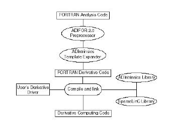
To retrieve the ADIFOR 2.0 automatic differentiation software for educational and non-profit research use, and for commercial evaluation, visit either of the ADIFOR group Web sites, at: http://www.mcs.anl.gov/adifor or http://www.cs.rice.edu/~adifor. These pages describe how to request access to ADIFOR 2.0 and download the software. The pages also contain links to publications related to ADIFOR, as well as legal notices.