Using the Aircraft Enhanced Tire Model
The Aircraft Enhanced Tire Model is comprised of the Adams Tire Fiala and UA (University of Arizona) tire models, with modifications that are necessary for aircraft landing gear analysis in Adams
This section contains information for using the Aircraft Enhanced Tire Model:
Overview
Assumptions
■Single contact point with the road profile.
■Disk representation of wheel and tire.
■User-controlled lateral and longitudinal deformation (vertical center of pressure shift) effects on tire center moments.
■First-order lag on longitudinal and lateral slip.
Inputs
The inputs to the Aircraft Enhanced Tire Model come from two sources:
■Input parameters from the tire property file (.tir), such as tire undeflected radius, that the tire references.
■Tire states, given through the tire interface with the solver, such as slip angle ( ).
).
). The following table summarizes the input data from the tire property file (.tir) that theAircraft Enhanced Tire Model requires.
Table 1 Aircraft Enhanced Tire Model Input Data
Parameters: | Description: |
|---|---|
[UNITS] block: LENGTH | Units of length for all tire property file values that involve length units. Valid entries: 'inch', 'cm', 'centimeter', 'foot', 'ft', 'kilometer', 'km', 'm', 'meter', 'mile', 'millimeter', 'mm'. |
[UNITS] block: FORCE | Units of force for all tire property file values that involve force units. Valid entries: 'dyne', 'kg_force', 'kilogram_force', 'knewton', 'kpound_force', 'lbf', 'millinewton', 'newton', 'ounce_force', 'pound_force'. |
[UNITS] block: MASS | Units of mass for all tire property file values that involve mass units. Valid entries: 'gram', 'kg', 'kilogram', 'kpound_mass', 'lbm', 'megagram', 'ounce_mass', 'pound_mass', 'slug'. |
[UNITS] block: ANGLE | Units of angle for all tire property file values that involve angle units. Valid entries: 'angular_minutes', 'am', 'angular_seconds', 'as', 'degree', 'deg', 'radian', 'rad'. |
[UNITS] block: TIME | Units of time for all tire property file values that involve time units. Valid entries: 'hour', 'millisecond', 'ms', 'minute', 'second', 'sec'. |
PROPERTY_FILE_FORMAT | Must be 'AIR_ENHANCED'. |
FUNCTION_NAME | Must be 'TYR1505'. |
HANDLING_MODE | 1 = don't compute handling forces (zero) 2 = Fiala-based handling force computations 3 = UATire-based handling force computations |
FRICTION_MODE | 1 = slip ratio-based friction coeff. model 2 = slip velocity-based friction coeff model A 3 = slip velocity-based friction coeff model B 4 = user-input custom Mu versus slip ratio See Friction Models (Fiala Handling Force Model) and Friction Models (University of Arizona (UA) Tire Handling Force Model). |
LAT_SLIP_MODE | 0 = lateral slip calculation without vertical tire speed effect (default) not 0 = lateral slip calculation with vertical tire speed effect |
UNLOADED RADIUS | Tire's outer radius under zero loading. (Units: length.) |
WIDTH | Tire's maximum undeflected (or unloaded) width. In simple geometry graphics, WIDTH represents the tread width, for visualization purposes only. In computations, however, WIDTH represents the tire's maximum undeflected width. (Units: length.) |
ASPECT_RATIO | Ratio of "rim-to-tread distance" to WIDTH. Used only for tire geometry graphics. (Units: none.) |
BOTTOMING_RADIUS (optional) | Wheel bottoming radius. (Units: length.) See Wheel Bottoming. |
VERTICAL_DAMPING | Vertical tire damping force coefficient. (Units: force/(length/time).) |
RELAXATION_LENGTH | Relaxation length. (Units: length.) See Transient Behavior. |
LOW_SPEED_DAMPING (optional) | The low speed damping rate when transient tire modelling is used (relaxation length not equal to zero). (Units: none.) See Transient Behavior. |
LOW_SPEED_THRESHOLD (optional) | The speed below which the low speed damping will be applied. (Units: length/time.) If not specified in the tire property file the value for this parameter is 4 m/s. See Transient Behavior. |
ROLLING_RESISTANCE | Rolling resistance moment coefficient, which represents the longitudinal shift in the vertical center of pressure, during pure rolling. (Units: length.) See Rolling Resistance Moment (Zero Handling Force Model) and Rolling Resistance Moment (University of Arizona ((UA) Tire Handling Force Model). |
CGAMMA | Tire's camber stiffness. Partial derivative of lateral force (Fy) with respect to inclination (camber) angle(  ) at zero camber angle. Used only if HANDLING_MODE = 3. (Units: force/force/angle.) ) at zero camber angle. Used only if HANDLING_MODE = 3. (Units: force/force/angle.)Note: If CGAMMA is less than or equal to 0, a value for CGAMMA is estimated. See Tire Operating Conditions. |
UMAX | Coefficient of friction at zero slip. (Units: none.) See Friction Models (Fiala Handling Force Model) and Friction Models (University of Arizona (UA) Tire Handling Force Model). |
UMIN | Coefficient of friction when tire is sliding. Not used if FRICTION_MODE = 2. (Units: none.) See Friction Models (Fiala Handling Force Model) and Friction Models (University of Arizona (UA) Tire Handling Force Model). |
V_UREF | Reference velocity for friction coefficient determination. Used only if FRICTION_MODE = 2 or 3. (Units: length/time.) See Friction Models (Fiala Handling Force Model) and Friction Models (University of Arizona (UA) Tire Handling Force Model). |
RR_DEFL_FACTOR | Factor used in the calculation of unbraked, unyawed tire rolling radius. (Units: none.) |
SLIP_STIFFNESS_FACTOR | Factor used in the calculation of slip stiffness, CSLIP,from longitudinal tire stiffness. (Units: none.) |
LON_DEFL_FACTOR | Reduction factor used in the calculation of longitudinal shift in the tire vertical center of pressure in the presence of a longitudinal force. (Units: none.) |
LAT_DEFL_FACTOR | Reduction factor used in the calculation of lateral shift in the tire vertical center of pressure in the presence of a lateral force. (Units: none.) |
[AIR_CURVE] block: pen | Column of tire/road penetration (deflection) values, corresponding to the adjacent tire radial force value. (Units: length.) |
[AIR_CURVE] block: fz | Column of tire radial force values, corresponding to the adjacent tire/road penetration (deflection) value. (Units: force.) |
[CORN_STIFFNESS] block: fz | Column of tire vertical load values, corresponding to the adjacent cornering stiffness value. (Units: force.) |
[CORN_STIFFNESS] block: c_alpha | Column of tire cornering stiffness values, corresponding to the adjacent tire vertical load value. (Units: force/angle.) |
[LON_STIFFNESS] block: fz | Column of tire vertical load values, corresponding to the adjacent longitudinal stiffness value. (Units: force.) |
[LON_STIFFNESS] block: lon_k | Column of tire longitudinal stiffness values, corresponding to the adjacent tire vertical load value. (Units: force/length.) |
[LAT_STIFFNESS] block: fz | Column of tire vertical load values, corresponding to the adjacent lateral stiffness value. (Units: force.) |
[LAT_STIFFNESS] block: lat_k | Column of tire lateral stiffness values, corresponding to the adjacent tire vertical load value. (Units: force/length.) |
[SHAPE] block: radial (optional) | Column of tire radial scale values, corresponding to the adjacent tire width station value. This value is multiplied with UNLOADED RADIUS. (Units: none.) See Tire Carcass Shape. |
[SHAPE] block: width (optional) | Column of tire width station values, corresponding to the adjacent radial scale value. 0.0 represents the tire centerline tread station and 1.0 represents the outermost tire tread station. Symmetry about the tire centerline is assumed. (Units: none.) See Tire Carcass Shape. |
[BOTTOMING_CURVE] block: pen (optional) | Column of rim/road penetration (deflection) values, corresponding to the adjacent rim radial force value. (Units: length.) See Wheel Bottoming. |
[BOTTOMING_CURVE] block: fz (optional) | Column of rim radial force values, corresponding to the adjacent rim/road penetration (deflection) value. (Units: force.) See Wheel Bottoming. |
Tire Property File Format Example
The following file, located in the shared database, is an example of the Aircraft Enhanced Tire Model tire property file:
install_dir/acar/shared_car_database.cdb/tires.tbl/AA_small_enha_relax.tir
where install_dir represents the location of the Adams installation directory.
Contact Methods
The Aircraft Enhanced Tire model supports all Adams Tire contact methods.
■One Point Follower Contact, used by default for 2D Road, 3D Spline Road, OpenCRG road and RGR Road.
■3D Equivalent Volume Contact, used by default for 3D Shell Road.
■3D Enveloping Contact, can be used with all road types when the keyword CONTACT_MODEL = '3D_ENVELOPING' is specified in the [MODEL] section of the tire property file.
The contact method supplies the tire model with the (effective) road height and road plane for the tire deflection/penetration calculation.
Wheel Bottoming
You can optionally supply a wheel bottoming deflection - load curve in the tire property file in the [BOTTOMING_CURVE] block. If the deflection of the wheel is so large that the rim will be hit (defined by the BOTTOMING_RADIUS parameter in the [DIMENSION] section of the tire property file), the tire vertical load will be increased according to the load curve defined in this section.
Note: | The rim-to-road contact algorithm is a simple penetration method (such as the 2D contact) based upon the tire-to-road contact calculation, which is strictly valid only for rather smooth road surfaces (the length of obstacles should have a wavelength longer than the tire circumference). The rim-to-road contact algorithm is not based on the 3D volume penetration method, but can be used in combination with the 3D Contact (that takes into account the volume penetration of the tire itself). If you omit the [BOTTOMING_CURVE] block from a tire property file, no force due to rim road contact will be added to the tire vertical force. |
The BOTTOMING_RADIUS may be chosen larger than the rim radius to account for the tire's material left in between the rim and the road, while the bottoming load-deflection curve may be adjusted for the change in stiffness.
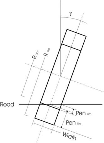
If (Pentire- (Rtire - Rbottom) - ½ width · | tan( ) |) < 0 the left or right side of the rim has contact with the road. Then the rim deflection Penrim can be calculated with:
) |) < 0 the left or right side of the rim has contact with the road. Then the rim deflection Penrim can be calculated with:■ = max(0 , ½width · | tan(
 ) | ) + Pentire- (Rtire - Rbottom) )
= max(0 , ½width · | tan() | ) + Pentire- (Rtire - Rbottom) )■Penrim=  /(2 · width · | tan(
 ) |)
) |)
/(2 · width · | tan() |)■Srim= ½width - max(width ,  | tan(
 ) |)/3
| tan() |)/3with Srim the lateral offset of the force with respect to the wheel plane.
If the full rim has contact with the road, the rim deflection is
■Penrim = Pentire- (Rtire - Rbottum)
■Srim= width2 · | tan( ) | · /(12· Penrim)
) | · /(12· Penrim)Using the load - deflection curve defined in the [BOTTOMING_CURVE] section of the tire property file, the additional vertical force due to the bottoming is calculated, while Srim multiplied by the sign of the inclination  is used to calculate the contribution of the bottoming force to the overturning moment. Further, the increase of the total wheel load Fz due to the bottoming (Fzrim) will not be taken into account in the calculation for Fx, Fy, My and Mz. The Fzrim will only contribute to the overtuning moment Mx using the Fzrim· Srim.
is used to calculate the contribution of the bottoming force to the overturning moment. Further, the increase of the total wheel load Fz due to the bottoming (Fzrim) will not be taken into account in the calculation for Fx, Fy, My and Mz. The Fzrim will only contribute to the overtuning moment Mx using the Fzrim· Srim.Note: | Rtire is equal to the unloaded tire radius, Pentire is similar to effpen. |
Normal Force of Road on Tire
The normal force of a road on a tire at the contact patch in the SAE coordinates (+Z downward) is always negative (directed upward). The normal force is:
Fz = min (0.0, {Fzk + Fzc}) + min (0.0, Fzrim)
where
■Fzk is the normal force due to the tire radial load-deflection curve
♦Fzk = - f (effpen, tire load-deflection spline)
■Fzc is the normal force due to tire vertical damping
♦Fzc = - VERTICAL_DAMPING x Vpen
■Fzrim is the normal force due to bottoming of the wheel
The normal penetration (effpen, or Δ) and penetration velocity (Vpen) are obtained from the appropriate road contact model.
Handling Forces of Road on Tire
The following topics are included:
Basic Tire Kinematics
All tire kinematic values are in the tire contact patch (SAE) reference system.
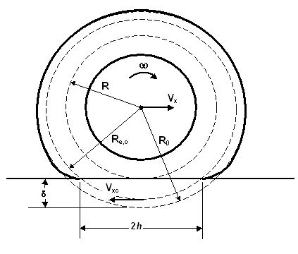
Figure 8 Unbraked, Unyawed, Effective Rolling Radius
Current Cornering Stiffness
The current cornering stiffness is a function of the current vertical load:
C = f(abs(Fz)), tire cornering stiffness versus vertical load spline
= f(abs(Fz)), tire cornering stiffness versus vertical load splineCurrent Longitudinal Stiffness
The current longitudinal stiffness is a function of the current vertical:
Klon = f(abs(Fz)), tire longitudinal stiffness versus vertical load spline
Current Lateral Stiffness
The current lateral stiffness is a function of the current vertical:
Klat = f(abs(Fz)), tire lateral stiffness versus vertical load spline
Current Longitudinal Slip Stiffness
The current longitudinal stiffness is a function of the current vertical:
CSLIP = Klon * UNLOADED_RADIUS * SLIP_STIFFNESS_FACTOR
Unloaded (and Ungrown) Radius
Ro = UNLOADED_RADIUS
Unloaded (and Ungrown) Diameter
Do = 2 * UNLOADED_RADIUS
Geometric Deflected Radius
R = UNLOADED_RADIUS - (effpen)
Effective Unbraked Rolling Radius
Re,o = UNLOADED_RADIUS - (effpen x RR_DEFL_FACTOR)
And RR_DEFL_FACTOR is usually set to 1/3.
And RR_DEFL_FACTOR is usually set to 1/3.
Wheel Carrier Translational Velocity
Vx, Vy, Vz
Total Rotational Velocity of Spinning Tire and Rotating Wheel Carrier

Contact Patch Rubber Velocity
Vxc = X-component of (  x
x  e,o)
e,o)
x e,o)where  e,o is the vertical radius vector of the scalar Re,o.
e,o is the vertical radius vector of the scalar Re,o.Vyc = Y-component of (  x
x  )
)
x )Vzc = Z-component of (  x
x  )
)
x )where  is the vertical radius vector of the scalar R.
is the vertical radius vector of the scalar R.Contact Patch Rubber Slip (or Scrub) Velocity
Vsx = Vx + Vxc
Vsy = Vy + Vyc if LAT_SLIP_MODE = 0
Vsy = Vy + Vyc + Vzc*tan( ) if LAT_SLIP_MODE = 1
) if LAT_SLIP_MODE = 1 The component Vzc* tan( ) takes into account the lateral slip due to a vertical movement of the tire if the roll inclination with the road is not zero. The default for LAT_SLIP_MODE is zero.
) takes into account the lateral slip due to a vertical movement of the tire if the roll inclination with the road is not zero. The default for LAT_SLIP_MODE is zero. Definition of Tire Slip Quantities
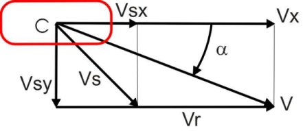
Figure 9 Slip Quantities at Combined Cornering and Braking/Traction
The longitudinal slip velocity Vsx in the SAE-axis system is defined using the longitudinal speed Vx, the wheel rotational velocity  , and the effective rolling radius Re:
, and the effective rolling radius Re:
The lateral slip velocity is equal to the lateral speed in the contact point with respect to the road plane:

The practical slip quantities  (longitudinal slip) and
  (slip angle) are calculated with these slip velocities in the contact point with:
(longitudinal slip) and (slip angle) are calculated with these slip velocities in the contact point with: and
and 
When the UA Tire is used for the force calculation the slip quantities during positive Vsx (driving) are defined as:
 and
and 
The rolling speed Vr is determined using the effective rolling radius Re:

Note that for realistic tire forces the slip angle  is limited to 45 deg and the longitudinal slip
  in between -1 (locked wheel) and 1.
is limited to 45 deg and the longitudinal slip in between -1 (locked wheel) and 1.Zero Handling Force Model
If this option is selected in the tire property file, friction and slip parameters are not used, and all handling forces will be zero:
Longitudinal Force
Fx = 0
Lateral Force
Fy = 0
Oversteering Moment
Tx = 0
Rolling Resistance Moment
Ty = 0
Aligning Moment
Tz = 0
Fiala Handling Force Model — Enhanced Tire
The Aircraft Basic Tire Model's Fiala Handling Force model is an extended Fiala model (Fiala, E., "Seitenkrafte am rollenden Luftreifen," VDI-Zeitschrift 96, 973 (1964)). This model provides reasonable results for simple maneuvers where inclination angle is not a major factor and where longitudinal and lateral slip effects may be considered unrelated.
Modifications are included to make the Fiala model more general and more appropriate for use in Adams.
Additional Parameters
Before calculating the current maximum available friction coefficient, the Fiala tire model requires the evaluation of some additional variables. First is the comprehensive slip S*s :
:
:S*s = (S2s + tan2(
 ))1/2
))1/2
= (S2s + tan2())1/2The truncated comprehensive slip (Ss ):
):
): S*s = min(1, S*s
 )
)
= min(1, S*s)Friction Models
You can choose from four friction models. The friction mode parameter within the tire property file is used to select the friction model. The friction model ultimately computes the maximum available comprehensive friction coefficient.
Slip Ratio-based Friction Model A (Linear U-Slip)
The resultant friction coefficient between the tire tread base and the terrain surface is determined as a function of the resultant comprehensive, truncated slip ratio (Ss ) and friction parameters (Umax and Umin). The friction parameters are experimentally obtained data representing the kinematic property between the surfaces of tire tread and the terrain.
) and friction parameters (Umax and Umin). The friction parameters are experimentally obtained data representing the kinematic property between the surfaces of tire tread and the terrain. A linear relationship between Ss and U(
 ), the corresponding maximum available road-tire friction coefficient, is assumed. The following figure shows this relationship.
and U(), the corresponding maximum available road-tire friction coefficient, is assumed. The following figure shows this relationship. 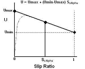
Figure 10 Linear Tire-Terrain Friction Model
Therefore, the current value coefficient of friction (U):
U = Umax + (Umin-Umax) x Ss
Note: | The figure illustrates that the available friction coefficient, U, varies linearly with slip ratio, but the actual curve of Fx/Fz is not linear, as described in Longitudinal Force. |
Slip (or Scrub) Velocity-based Friction Decay Model A
The resultant friction coefficient between the tire tread base and the terrain surface is determined as a function of the total planar slip (or scrubbing) velocity Vsxy, maximum friction parameter (Umax), and the friction coefficient reference velocity parameter V_UREF from the tire property file. The friction parameters are experimentally obtained data representing the kinematic property between the surfaces of tire tread and the terrain.
A decay relationship between Vsxy and U ( ), the corresponding maximum available road-tire friction coefficient, is assumed. The following figure shows this relationship.
), the corresponding maximum available road-tire friction coefficient, is assumed. The following figure shows this relationship. 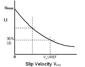
Figure 11 Friction Decay Model A
Therefore, the current value coefficient of friction (U):
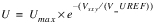
Notice that Umin is not used in this friction model. Also, notice the effect of V_UREF upon the decay of the available friction coefficient with total slip (or scrub) velocity Vsxy:
♦If Vsxy = 0, then U = Umax
♦If Vsxy = V_UREF/2, then U = 60.7% of Umax
♦If Vsxy = V_UREF, then U = 36.78% of Umax
Note: | The figure illustrates the available friction coefficient, U, as it varies with slip ratio. The actual curve of Fx/Fz deviates from this curve, as described in Longitudinal Force. |
Slip (or Scrub) Velocity-based Friction Decay Model B
The resultant friction coefficient between the tire tread base and the terrain surface is determined as a function of the total planar slip (or scrubbing) velocity Vsxy, friction parameters (Umax and Umin), and the friction coefficient reference velocity parameter V_UREF from the tire property file. The friction parameters are experimentally obtained data representing the kinematic property between the surfaces of tire tread and the terrain.
A decay relationship between Vsxy and U ( ), the corresponding maximum available road-tire friction coefficient, is assumed (AGARD-R-800 "The Design, Qualification and Maintenance of Vibration-Free Landing Gear": Denti, E., Fanteria D., "Analysis and Control of the Flexible Dynamics of Landing Gear in the Presence of Antiskid Control Systems" (1996)). The following figure shows this relationship.
), the corresponding maximum available road-tire friction coefficient, is assumed (AGARD-R-800 "The Design, Qualification and Maintenance of Vibration-Free Landing Gear": Denti, E., Fanteria D., "Analysis and Control of the Flexible Dynamics of Landing Gear in the Presence of Antiskid Control Systems" (1996)). The following figure shows this relationship. 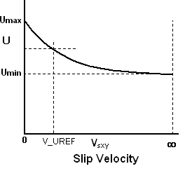
Figure 12 Friction Decay Model B
Therefore, the current value coefficient of friction (U):
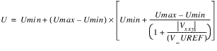
Notice the effect of V_UREF on the decay of the available friction coefficient with total slip (or scrub) velocity Vsxy:
■If Vsxy = 0, then U = Umax
■If Vsxy = V_UREF, then U = Average of Umax and Umin
■If Vsxy = , then U = Umin
, then U = Umin Note: | The figure illustrates the available friction coefficient, U, as it varies with slip ratio. The actual curve of Fx/Fz deviates from this curve, as described in Longitudinal Force. |
Slip Ratio based Model B (User-Defined Mu-Slip)
The resultant friction coefficient between the tire tread base and the terrain surface is determined as a function of the resultant comprehensive, truncated slip ratio (Ss ) and a user-defined table of U (
 ). The tabular data are experimentally obtained and represent the kinematic property between the surfaces of tire tread and the terrain.
) and a user-defined table of U (). The tabular data are experimentally obtained and represent the kinematic property between the surfaces of tire tread and the terrain. The following figure shows the relationship between Ss and U (
 ), the corresponding maximum available road-tire friction coefficient.
and U (), the corresponding maximum available road-tire friction coefficient. 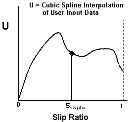
Figure 13 User-Defined Fiala Tire-Terrain Friction Model
Therefore, the current value coefficient of friction (U):
U = a cubic spline interpolation of U versus Ss curve
curve
curveAdd a section called [MU_SLIP_CURVE] to the tire property file, in a similar way as for example, [RIMPACT_CURVE] shown in the example tire property file acar/shared_car_database.cdb/tires.tbl/AA_small_basic_relax.tir, to represent the mu versus slip ratio data.
Note: | The figure illustrates the available friction coefficient, U, as it varies with slip ratio. The actual curve of Fx/Fz deviates from this curve, as described in Longitudinal Force. |
Handling Force Evaluation
Now that the current maximum available total friction coefficient U is known, the Fiala handling forces can be calculated.
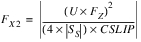
Longitudinal Force
The longitudinal force depends on the vertical force (Fz), the current maximum available total coefficient of friction (U), and the longitudinal slip ratio (Ss).
Fiala defines a critical longitudinal slip (S_critical):
S_critical = 
This is the value of longitudinal slip beyond which the tire is sliding.
Case 1. Elastic Deformation State:|Ss| < S_critical
Case 2. Complete Sliding State: |Ss| > S_critical
Fx = -sign(Ss)(Fx1-Fx2)
where:
■Fx1 = U x Fz
■
The calculations of Fx can be used to calculate Fx/Fz, which can be contrasted to the available total coefficient of friction (U) curves shown above. All of the above figures are plots of U, but they are not the plots of Fx/Fz. The U curves show the maximum possible friction coefficient, but the actual longitudinal force, while based on U, is modified by the rolling characteristics of the tire.
For example, consider the plot of Linear Fiala Tire-Terrain Friction Model. The coefficient of friction is a straight line. Consider next the following figure based on the equations for Fx shown in Case 1 and Case 2 above. The following figure, created using arbitrarily chosen parameters, illustrates that Fx/Fz is less than the value of U at every value of slip, Ss , The actual Fx/Fz curve is a function of the U curve, CSLIP, and tire vertical force, Fz.
, The actual Fx/Fz curve is a function of the U curve, CSLIP, and tire vertical force, Fz. 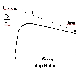
This type of difference between the chosen U curve and Fx/Fz affects all four friction models. You should keep this in mind when creating your tire property file. Also, after you run a simulation, such as a braking or wheel test simulation, you can plot Fx/Fz to determine whether the friction values are what you require.
Lateral Force
Like the longitudinal force, the lateral force depends on the vertical force (Fz) and the current coefficient of friction (U). And similar to the longitudinal force calculation, Fiala defines a critical lateral slip (Alpha_critical):
Alpha_critical = arctan 
The lateral force peaks at a value equal to U x |Fz| when the slip angle (Alpha) equals the critical slip angle (Alpha_critical).
Case 1. Elastic Deformation State: 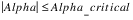
Fy = - U x |Fz| x (1-H3) x sign(Alpha)
where: 
Case 2. Sliding State: |Alpha| > Alpha_critical
Fy = -U|Fz|sign(Alpha)
Oversteering Moment
Tx = 0
Rolling Resistance Moment
When the tire is rolling forward: Ty = -ROLLING_RESISTANCE * Fz
When the tire is rolling backward: Ty = ROLLING_RESISTANCE * Fz
Aligning Moment
Case 1. Elastic Deformation State: 

Case 2. Complete Sliding State: |Alpha| > Alpha_critical
Tz= 0.0
University of Arizona (UA) Tire Handling Force Model - Enhanced Tire
The Aircraft Enhanced Tire Model's UA Tire Handling Force model is an extension of the University of Arizona tire model, recently developed by Drs. P.E. Nikravesh and G. Gim (Gim, Gwanghun, "Vehicle Dynamic Simulation with a Comprehensive Model for Pneumatic Tires," Ph.D. Thesis, The University of Arizona (1988)). This analytical model has been extensively tested and verified against experimental data and other analytical models. Please note that the current implementation of the University of Arizona tire model uses a friction circle rather than the original friction ellipse. The ellipse caused undesirable results under some circumstances due to its dependence on the integration time step.
Modifications are included to make the UA Tire model more general and more appropriate for use in Adams.
Additional Parameters
The UATire tire model requires the evaluation of some additional variables:
Lateral Slip Ratios
The lateral slip ratio due to slip angle,  , may then be defined as:
, may then be defined as:  whether traction or braking
The lateral slip ratio due to inclination angle,  , is defined as:
, is defined as:
A combined lateral slip ratio due to slip and inclination angles,  , is defined as:
, is defined as: whether traction or braking
where  is the length of the contact patch.
is the length of the contact patch.
Comprehensive Slip Ratio
A comprehensive slip ratio due to slip ratio, slip angle, and inclination angle may be defined as:
Note that:
 for
for 
 for
for 
 for
for 
 for
for 
Now a slip velocity directional angle  may be defined as:
may be defined as:
Slip properties and slip ratio relationships are shown in the following figure (a), (b), and (c):
a. Slip Properties Between Tire and Terrain During Braking
b. Slip Properties Between Tire and Terrain During Traction
c. Resultant Slip Ratio Relationships
Friction Models
You can choose from three friction models. The friction mode parameter within the tire property file is used to select the friction model. The friction model ultimately computes the maximum available comprehensive friction coefficient
Slip Ratio-based Friction Model
The resultant friction coefficient between the tire tread base and the terrain surface is determined as a function of the resultant comprehensive, truncated slip ratio ( ) and friction parameters (U0 and U1). The friction parameters are experimentally obtained data representing the kinematic property between the surfaces of tire tread and the terrain.
) and friction parameters (U0 and U1). The friction parameters are experimentally obtained data representing the kinematic property between the surfaces of tire tread and the terrain.A linear relationship between  and
and  , the corresponding maximum available road-tire friction coefficient, is assumed. The following figure shows this relationship.
and , the corresponding maximum available road-tire friction coefficient, is assumed. The following figure shows this relationship.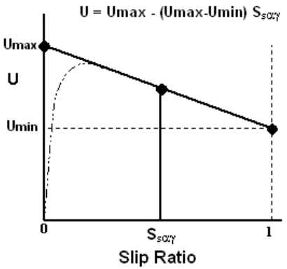
Figure 14 Linear UATire Tire-Terrain Friction Model
Therefore, the current value coefficient of friction (U) is:
U = Umax - (Umax-Umin) x 
Slip (or Scrub) Velocity-based Friction Decay Model A
The resultant friction coefficient between the tire tread base and the terrain surface is determined as a function of the total planar slip (or scrubbing) velocity Vsxy , maximum friction parameter (Umax), and the friction coefficient reference velocity parameter V_UREF from the tire property file. The friction parameters are experimentally obtained data representing the kinematic property between the surfaces of tire tread and the terrain.
A decay relationship between Vsxy and  , the corresponding maximum available road-tire friction coefficient, is assumed. The following figure shows this relationship.
, the corresponding maximum available road-tire friction coefficient, is assumed. The following figure shows this relationship.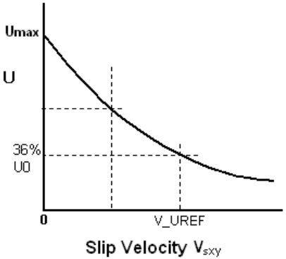
Figure 15 Friction Decay Model A
Therefore, the current value coefficient of friction (U):
Notice that Umin is not used in this friction model. Also, notice the effect of V_UREF upon the decay of the available friction coefficient with total slip (or scrub) velocity Vsxy:
■If Vsxy = 0 , then U = Umax
■If Vsxy = V_UREF/2 , then U = 60.7% of Umax
■If Vsxy = V_UREF, then U = 36.78% of Umax
Slip (or Scrub) Velocity-based Friction Decay Model B
The resultant friction coefficient between the tire tread base and the terrain surface is determined as a function of the total planar slip (or scrubbing) velocity Vsxy, friction parameters (Umax and Umin), and the friction coefficient reference velocity parameter V_UREF from the tire property file. The friction parameters are experimentally obtained data representing the kinematic property between the surfaces of tire tread and the terrain.
A decay relationship between Vsxy and  , the corresponding maximum available road-tire friction coefficient, is assume, from (Denti, E., Fanteria D., "Analysis and Control of the Flexible Dynamics of Landing Gear in the Presence of Antiskid Control Systems" AGARD-R-800 "The Design, Qualification and Maintenance of Vibration-Free Landing Gear" (1996)). The following figure shows this relationship.
, the corresponding maximum available road-tire friction coefficient, is assume, from (Denti, E., Fanteria D., "Analysis and Control of the Flexible Dynamics of Landing Gear in the Presence of Antiskid Control Systems" AGARD-R-800 "The Design, Qualification and Maintenance of Vibration-Free Landing Gear" (1996)). The following figure shows this relationship.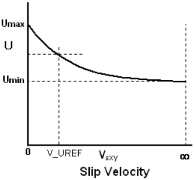
Figure 16 Friction Decay Model B
Therefore, the current value coefficient of friction (U) is:
Notice the effect of V_UREF upon the decay of the available friction coefficient with total slip (or scrub) velocity Vsxy:
■If Vsxy = 0, then U = Umax
■If Vsxy = V_UREF , then U = Average of Umax and Umin
■If Vsxy =  , then U = Umin
, then U = UminFriction Circle Concept
In the UATire model, the friction circle concept allows for different values of longitudinal and lateral friction coefficients ( and
and  ) but limits the maximum value for both coefficients to
  . The relationship that defines the friction circle follows:
and ) but limits the maximum value for both coefficients to . The relationship that defines the friction circle follows:
or 
and 
where 
Note that  and
and  in the following figure depend on the untruncated value
  .
.
and in the following figure depend on the untruncated value .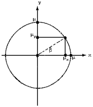
Figure 17 Friction Circle Concept
Tire Operating Conditions
To compute longitudinal force, lateral force, and self-aligning torque in the SAE coordinate system, you must perform a test to determine the precise operating conditions. The conditions of interest are:

 and
and 
 and
and 
Note: | Cs = CSLIP ,  = CALPHA and = CALPHA and  = CGAMMA = CGAMMA |
If  then a camber stiffness is estimated using:
then a camber stiffness is estimated using:
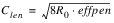
with Clen the contact length is estimated by:
The lateral force Fh can be decomposed into two components: Fha and Fhg. The two components are in the same direction if  and in opposite direction if
  .
.
and in opposite direction if .Case 1. 
Before computing the longitudinal force, the lateral force, and the self-aligning torque, some slip parameters and a modified lateral friction coefficient should be determined. If a slip ratio due to the critical inclination angle is denoted by  , then it can be evaluated as:
, then it can be evaluated as:
If Ssc represents a slip ratio due to the critical (longitudinal) slip ratio, then it can be evaluated as:

If a slip ratio due to the critical slip angle is denoted by  , then it can be determined as
, then it can be determined as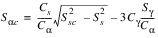
when Ss < Ssc.
The term "critical" stands for the maximum value which allows an elastic deformation of a tire during pure slip due to pure slip ratio, slip angle, or inclination angle. Whenever any slip ratio becomes greater than its corresponding critical value, an elastic deformation no longer exists, but instead complete sliding state represents the contact condition between the tire tread base and the terrain surface.
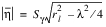
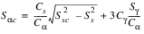
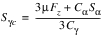
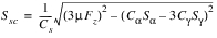
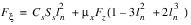
A nondimensional slip ratio Sn is determined as:

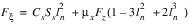
where:
■B1 = (3mFz)2 - (3CγSγ)2
■B2 = -3CαSαCγSγ
■B3 = -[(CsSs)2 + (CαSα)2]
A nondimensional contact patch length is determined as:
ln = 1 - Sn
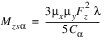
A modified lateral friction coefficient  is evaluated as:
is evaluated as: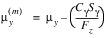
where  is the available friction as determined by the friction circle.
is the available friction as determined by the friction circle.To determine the longitudinal force, the lateral force, and the self-aligning torque, consider two subcases separately. The first case is for the elastic deformation state, while the other is for the complete sliding state without any elastic deformation of a tire. These two subcases are distinguished by slip ratios caused by the critical values of the slip ratio, the slip angle, and the inclination angle. Specifically, if all of slip ratios are smaller than those of their corresponding critical values, then there exists an elastic deformation state, otherwise there exists only complete sliding state between the tire tread base and the terrain surface.
1. Elastic Deformation State:  ,
,  and
and 
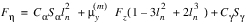
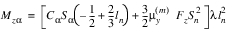
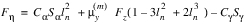
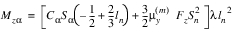
, and In the elastic deformation state, the longitudinal force  , the lateral force Fη, and three components of the self-aligning torque are written as functions of the elastic stiffness and the slip ratio as well as the normal force and the friction coefficients, such as:
, the lateral force Fη, and three components of the self-aligning torque are written as functions of the elastic stiffness and the slip ratio as well as the normal force and the friction coefficients, such as: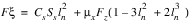


where:
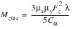
■ is the offset between the wheel plane center and the tire tread base.
is the offset between the wheel plane center and the tire tread base.■ is set to zero if it is negative.
is set to zero if it is negative.■ is the portion of the self-aligning torque generated by the slip angle a.
is the portion of the self-aligning torque generated by the slip angle a.■ and
and  are other components of the self-aligning torque produced by the longitudinal force, which has an offset between the wheel center plane and the tire tread base, due to the slip angle a and the inclination angle g, respectively. The self-aligning torque Mz is determined as combinations of
  ,
,  and
and  .
.
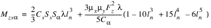
and are other components of the self-aligning torque produced by the longitudinal force, which has an offset between the wheel center plane and the tire tread base, due to the slip angle a and the inclination angle g, respectively. The self-aligning torque Mz is determined as combinations of , and . 2. Complete Sliding State: Sg > Sgc, Ss > Ssc or Sa > Sac
In the complete sliding state, the longitudinal force, the lateral force, and three components of the self-aligning torque are determined as functions of the normal force and the friction coefficients without any elastic stiffness and slip ratio as:


Case 2:  and
and 
and Same as in Case 1, a slip ratio due to the critical value of the slip ratio can be obtained as:

A slip ratio due to the critical value of the slip angle can be found as:
when Ss < Ssc.
The nondimensional slip ratio Sn, is determined as:

where:
■B1 = (3mFz)2 - (3CγSγ)2
■B2 = -3CαSαCγSγ
■B3 = -[(CsSs)2 + (CαSα)2]
The nondimensional contact patch length ln is found from the equation ln = 1 - Sn, and the modified lateral friction coefficient  is expressed as:
is expressed as:
For the longitudinal force, the lateral force, and the self-aligning torque two subcases should also be considered separately. A slip ratio due to the critical value of the inclination angle is not needed here since the required condition for Case 2, CαSα > CγSγ, replaces the critical condition of the inclination angle.
1. Elastic Deformation State: Ss < Ssc and Sa < Sac
In the elastic deformation state:

2. Complete sliding state: Ss > Ssc or Sa > Sac


Case 3:  and
and 
and Similar to cases 1 and 2, slip ratios due to the critical values of the inclination angle and the slip ratio are obtained as:
The nondimensional slip ratio Sn, is expressed as:
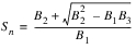
where:
■B1 = (3mFz)2 - (3CγSγ)2
■B2 = -3CαSαCγSγ
■B3 = -[(CsSs)2 + (CαSα)2]
For the longitudinal force, the lateral force, and the self-aligning torque, two subcases should also be considered similar to Cases 1 and 2. A slip ratio due to the critical value of the slip angle is not needed here since the required condition for Case 3, CαSα< CγSγ, replaces the critical condition of the slip angle.
1. Elastic Deformation State: Sg < Sgc and Ss < Ssc
In the elastic deformation state, Fh and Mza may be written:


2. Complete Sliding State: Sg > Sgc or Ss > Ssc
In the complete sliding state,  , Fh, Mza, Mzsa, and Mzsg can be determined by using:
, Fh, Mza, Mzsa, and Mzsg can be determined by using:


respectively. The longitudinal force  , the lateral force Fη, and three components of the self-aligning torques Mza, Mzsa, and Mzsg always have positive values, but they can be transformed to have positive or negative values depending on the slip ratio σ, the slip angle α, and the inclination angle γ in the SAE coordinate system.
, the lateral force Fη, and three components of the self-aligning torques Mza, Mzsa, and Mzsg always have positive values, but they can be transformed to have positive or negative values depending on the slip ratio σ, the slip angle α, and the inclination angle γ in the SAE coordinate system.Tire Handling Forces and Moments in the SAE Coordinate System
For the general formulations of the longitudinal force Fx, lateral force Fy, and self-aligning torque Mz, in the SAE coordinate system (see the figure, SAE Tire Coordinate System), the three possible combinations of the slip ratio, the slip angle, and the inclination angle are also considered.
Longitudinal Force
Fx = -sign(s) Fx, for all cases
Lateral Force
Fy = -sign(a) Fh, for cases 1 and 2
Fy = sign(g) Fh, for case 3
Self-aligning Torque
Mz = sign(a) Mza + sign(s) [-sign(a) Mzsa + sign(g)Mzsg]
Rolling Resistance Moment
My = -Cr Fz, for a forward rolling tire
My = Cr Fz, for a backward rolling tire
Where Cr = ROLLING_RESISTANCE.
Moment Adjustments
An adjustment to the tire moments is conducted to capture the effects of the longitudinal and lateral shifting of the approximate contact patch vertical center of pressure and center of longitudinal shear pressure, in the presence of longitudinal and lateral tire forces.
Note: | A separate moment adjustment has previously been calculated for the tire rolling resistance effects. |
Longitudinal Center of Pressure Shift
dlon = Fx / [max(1,abs(Klon)] * LON_DEFL_FACTOR
Lateral Center of Pressure Shift
dlat = Fy / [max(1,abs(Klat)] * LAT_DEFL_FACTOR
Moment Adjustments
Mx = Mx + [ Fz * dlat]
My = My - [ Fz * dlon]
Mz = Mz - [ Fx * dlat]
Force Reducer
In a balancing simulation, you can switch on the force reducer by using the tire user array. If the first element reads the value 1500 and the second 1, the force reducer is switched on. Except for the vertical load Fz, all tire forces and moments are reduced drastically to reach airplane equilibrium in a more efficient way.
Fx = Fx * FORCE_REDUCER_X
Fy = Fy * FORCE_REDUCER_Y
Mx = Mx * FORCE_REDUCER_Y
My = My * FORCE_REDUCER_X
Mx = Mz* FORCE_REDUCER_Y
FORCE_REDUCER_X = 0.01
FORCE_REDUCER_Y = 0.0
Fy = Fy * FORCE_REDUCER_Y
Mx = Mx * FORCE_REDUCER_Y
My = My * FORCE_REDUCER_X
Mx = Mz* FORCE_REDUCER_Y
FORCE_REDUCER_X = 0.01
FORCE_REDUCER_Y = 0.0
Transient Behavior
In the upper sections described force calculations are valid for the 'so-called' steady-state tire response, in other words tire dynamics is not taken into account. However, in general, the tire will be exposed to changes of input in terms of vertical load and longitudinal and lateral slip continuously.
For estimating transient tire behavior, a linear transient model is used as described in [1].
In the linear transient model the tire contact point S' is suspended to the wheel-rim plane with a longitudinal and lateral spring, with respectively stiffness's CFx and CFy. In the figure below a top view of the tire with the single contact point S' and the longitudinal (u) and lateral (v) carcass deflections is shown.
The contact point may move with respect to the wheel-rim plane and road. Movements relative to the road will result in tire-road interaction forces. Differences in slip velocities at point S and point S' will result in the tire carcass to deflect. The change of the longitudinal deflection u can be defined as:
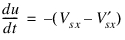
and the lateral deflection v as:
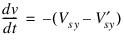
For small values of slip the side force Fy can be calculated using the cornering stiffness CFα as follows:
While the lateral force on the carcass reads:

When introducing the lateral relaxation length σα as:

For Air Basic Tire, the relaxation σ is equal to the relaxation as specified in the tire property file.
For Air Enhance Tire, the relaxation σ is corrected with the footprint length:
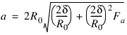
■a is half the footprint length
■R0 the unloaded tire radius
■δ the tire deflection
■Fa the footprint length factor
The relaxation for Air Enhance is then:

With  the relaxation value specified in the tire property file.
the relaxation value specified in the tire property file.the differential equation for the lateral deflection can be written as follows:
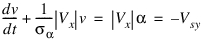
For linear small slip we can define the practical slip quantity α' as:
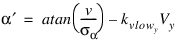
With α' the equation for the lateral deflection becomes:
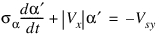
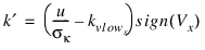
Similar the differential equation for longitudinal direction with the longitudinal relaxation length σκ can be derived:
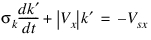
with the practical slip quantity 
These practical slip quantities  and
and  are used instead of the usual
  and
and  definitions for steady-state tire behavior.
and are used instead of the usual and definitions for steady-state tire behavior.  and
and  optional the damping rates that can be applied to achieve more damping at low speeds (below the LOW_SPEED_THRESHOLD value). The LOW_SPEED_DAMPING parameter in the tire property file yields:
 = 100 ·
  = LOW_SPEED_DAMPING
The longitudinal and lateral relaxation length are read from the tire property file, see Tire Property File Format Example.
Note that in transient mode the tire model is able to deal with zero speed (stand-still), because this linear transient model works with tire deflections instead of slip velocities. The effective lateral compliance of the tire at stand-still in transient mode is:

And similar in longitudinal direction the compliance is:

Note: | If the tire property file's REL_LEN_LON or REL_LEN_LAT = 0, then steady-state tire behavior is calculated. |
Reference
1. H.B. Pacejka, Tyre and Vehicle Dynamics, 2002, Butterworth-Heinemann, ISBN 0 7506 5141.