Linearization in Adams Vibration
Nonlinear Adams models are represented by implicit equations of the form:
 | (1) |
where:
■z = vector of states of the model.
■G = system of first-order differential and algebraic equations.
The states of the model include:
■Displacement and velocity states from mass-bearing elements PART, POINT_MASS, and FLEX_BODY
■First-order states introduced by the DIFF, LSE, GSE, and TFSISO modeling elements
■Forces variables due to force elements (SFORCE, VFORCE and so on)
■Lagrange multipliers due to kinematic constraints (JOINT, JPRIM, MOTION, PTCV and CVCV)
■Variables defined in the model (VARIABLE).
This system of equations is linearized about an operating point z0. An operating point is defined by an initial-conditions analysis or static or dynamic analysis [Sohoni, 1986; Negrut and Ortiz, 2005]. Using a process of eliminating algebraic equations from the linearized representation of, ordinary differential equations along with algebraic output equations of the following state-space form are obtained:
 | (2) |
where:
■x = Vector of states of the linear model (a subset of vector z above)
■y = Outputs from the linear model (defined with POUTPUT statements or output channels in the graphical interface.)
■u = Inputs to the linear model (defined with PINPUT statements or input channels in the graphical interface.)
■A,B,C,D = Real state matrices for the linear model computed by the linearization algorithm.
Specific details of the linearization process implemented in Adams Solver (FORTRAN) are given by Sohoni [1986]. Negrut and Ortiz [2005] have given details of linearization process implemented in Adams Solver (C++).
States of the linear model, x in equation (2) are a subset of states of the nonlinear model, represented by z in (1). When performing normal-modes analysis, specification of inputs and outputs is not required. Therefore, the problem is reduced to finding a solution to the homogeneous equation:
 | (3) |
Representing the solution to equation (3) as:

where:
■ = ith eigenvector
= ith eigenvector ■ = ith eigenvalue
= ith eigenvalueSubstituting in equation (3) gives:
 | (4) |
Equation (4) is the classic eigenvalue problem. This problem is solved in Adams Vibration using the well-known QR method [Press et. al., 1994] for computing eigenvalues and eigenvectors. The A matrix includes all damping effects in the model, however the damping terms are set to zero when the user selects the no damping option.
Note that Adams Vibration always computes  and
and  as complex quantities (complex eigensolution). The complete eigensolution to equation (4) includes a modal matrix (matrix of mode shapes) and a vector of eigenvalues.
and as complex quantities (complex eigensolution). The complete eigensolution to equation (4) includes a modal matrix (matrix of mode shapes) and a vector of eigenvalues. Each eigenvalue has the form:
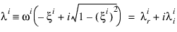
where:
■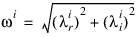 is the ith natural frequency.
is the ith natural frequency.■
Differences between proportional and general viscous damping – Adams Vibration implements general viscous damping. In these cases, the internally computed damping matrix is no longer proportional to mass and/or stiffness matrices. Adams Vibration always uses a complex eigenvalue solution.
Forced Response Analysis
Inputs and outputs to the linear model are defined by means of input and output channels in Adams Vibration. Input channels contribute to the B matrix. Output channels contribute to the C matrix. The D matrix represents direct interaction between input and output channels. For more details, see Modeling of Vibration Entities.
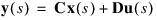
Using Laplace transform, equation (2) can be expressed in the form [De Silva, 2000]:
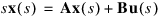 | (5) |
where:
■s = Laplace variable
■x(s), u(s), y(s) are the Laplace transforms of the state vector, inputs and outputs respectively.
From equation (5), the transfer function in the state-space form is given as:
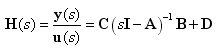 | (6) |
Transformation to Modal Space
Using the model eigenvectors as a basis for the solution, equation (5) is transformed to modal space using the modal transformation:
 | (7) |
where:
■Z = Matrix of eigenvectors
■q(s) = Array of modal coordinates
The ith column of Ζ corresponds to eigenvector  of the model.
of the model.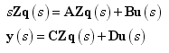 | (8) |
Simplifying equation (8) gives:
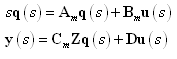 | (9) |
where:
■
■
■
Therefore, the transfer function for the model in modal space is given as:
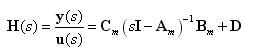 | (10) |
When asking for the transfer function of a model, you specify the range of values for s and the number of steps. At each step in the range of s, transfer function H(s) is computed from the expression in the right-hand side of equation (10).
Transfer functions can be computed in two ways, that is, using equation (6) or equation (10). Solution of the transfer function in the form of equation (6) is called the direct solution, while solution in the form equation (10) is called the modal solution.
Adams Vibration uses the following steps to compute the transfer function for the model:
1. Get the given input/output channel specifications.
2. Compute state matrices in the state-space form as in equation (2).
3. Compute the complex eigensolution for the model using equation (4).
4. Transform to modal space using equation (9).
5. Compute transfer function from equation (10).
Due to degeneracy in the eigensolution, for some models, Z may not be invertible. In such cases, the transfer function is computed using the direct solution of equation (6). The modal solution for transfer function computation is much faster than the direct solution. If the transfer function is computed using the direct method, it will not be possible to plot modal coordinates and participations or perform vibration animation for the model. However, normal mode shapes can still be animated.