Vibration Analyses
Adams Vibration performs two types of vibration analyses:
■Normal Mode Analysis to compute eigenvalues and eigenvectors for a model
■Forced Vibration Analysis to compute the forced response of the model to vibratory inputs applied using vibration input channels and actuators on the model. Eigenvalues and eigenvectors are also available computed during the forced response analysis.
Normal Mode Analysis
The linearization of the equations of motion of a complex Adams system including coupled differential equations, variable definitions, force definitions, controls systems and output equations is performed using the algorithm in [Sohoni et al., 1986] when using the Adams FORTRAN Solver or the algorithm in [Negrut et al., 2005] when using the Adams C++ Solver.
In either case, the linearized equations for the full system take the following form:

This linear representation is known as the minimal state-space representation or as the input/output equations. Matrix A is called the linearization matrix and matrices B, C, and D have different names in the technical literature. In general, vector X includes displacements, velocities and differential states of the model.
 .
.Vector q includes a subset of all of the displacement states in the system while vector v is the corresponding set of velocities. Vectors q and v are of the same size. Vector z includes all of the differential states defined in the system. The z states are the results of DIFF, LSE, TFSISO, or GSE elements included in the model (those elements define ordinary differential equations coupled with the mechanical system). Notice that vector q may include a set of user-defined coordinates when using the Adams C++ Solver. The above references describe the selection algorithm for the states in q. Adams Vibration, Adams Linear and the stand-alone version of Adams Solver all provide tools to export the A, B, C, D matrices and the list of linearization coordinates q, z, v, using two different file formats in ASCII form. Notice vector q includes neither Lagrange multipliers nor force/variable definitions.
Vector u stands for inputs to the system. For the homogenous case (u=0) and no output equations, the state-space representation reduces to:
 | (11) |
Simple case of no differential states
For clarity, consider first the case with no differential states in the Adams model, hence vector X takes the form:
 | (12) |
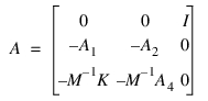
In this case, the linearization matrix A takes this form:
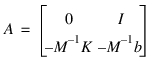 | (13) |
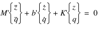
Here M, K and b are matrices that may not be symmetric. I is the identity matrix. Using Equations (12) and (13) into Equation (11), and simplifying we obtain:
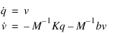
These two equations combined reduce to the well-known form:
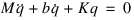 | (14) |
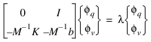
Equation (14) is called the MKB representation and matrices M, b and K can be exported using Adams Linear into different file formats. Instead of performing a modal analysis using Equation (14), Adams Vibration solves a complex eigenvalue problem using Equations (11) as the starting point. Representing the solution as:

Equation (11) transforms into a standard eigenvalue problem:
 | (15) |
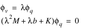
Adams Vibration uses a complex eigenvalue solution algorithm to compute eigenvalues  and mode shapes
  . In general, matrix A is non-symmetric and, in many cases, it can be ill conditioned or even singular. Hence, mode shapes are not orthogonal. See [Meyer, 2000] for a complete set of properties and theorems related to the eigensystem shown in Equation (15).
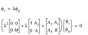
and mode shapes . In general, matrix A is non-symmetric and, in many cases, it can be ill conditioned or even singular. Hence, mode shapes are not orthogonal. See [Meyer, 2000] for a complete set of properties and theorems related to the eigensystem shown in Equation (15).For the simple case defined by Equations (12), (13) and (14), there is an important property related the computed mode shapes. A typical mode shape of the simple system can be split into:
 | (16) |
After making simplifications, we obtain:
 | (17) |
However, matrices M, b and K need not be symmetric, hence orthogonality properties do not apply.
General case with differential states
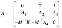
For the case of Adams models that do have differential states, vector X and the A matrix take the general forms:
 | (18) |
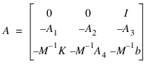 | (19) |
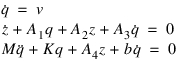
The last two equations can be rewritten as:
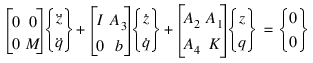 | (20) |
or
 | (21) |
Equation (21) is the MKB representation for the general system and, as above, matrices M', b', and K' can be computed and exported using Adams Linear.
For the general case of Equation (19) the eigensolution will compute the eigenvalues and mode shapes using the same algorithm used for the simple model with no differential states. Similarly, the linearization matrix A is not symmetric and the orthogonality conditions do not apply except for very special cases. Defining a generic mode shape as:
 | (22) |
 | (23) |
Eigensolution
Adams Vibration will compute eigenvalues of matrix A using a QR algorithm regardless of the type of model. We emphasize that the A matrix is, in general, non-symmetric, hence all orthogonality theorems for computed mode shapes do not apply. Moreover, the A matrix does not need to be full rank nor well conditioned. Adams models with control systems or in singular configurations (for example, neutral static equilibrium, bifurcation points and so on) may exhibit multiple zero value eigenvalues or large real eigenvalues.
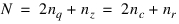
In the general case, the size of the A matrix is:
 | (24) |
Where nq is the size of the q vector (vectors q and v are of the same size) and nz is the size of the z vector. The eigensolution will compute a set of nr real eigenvalues and 2nc complex eigenvalues (all complex eigenvalues form a set of conjugate pairs). Therefore:
 | (25) |
Notice that Adams Vibration will only display a table with nc+nr eigenvalues only (conjugate complex values are not displayed). See Eigenvalue Table Reported in Adams View for an example output using the Adams Vibration user interface. Notice in the example in Table 1, there are 2 real-only eigenvalues and 2 complex eigenvalues. Hence the size of the A matrix is 2*2+2=6.
By default the eigensolution is performed on the full computed A matrix. Hence, all damping properties in the system are taken into account. If you want to compute the eigensolution without the damping properties, then uncheck the Damping checkbox in the Perform Vibrational Analysis dialog box.
A very important notice is due here. If you use the Adams Solver C++, and if you uncheck the Damping checkbox, Adams Vibration will set matrix b to zero in Equation (19) to get:
 | (26) |
However, if you use the Adams Solver FORTRAN, and you uncheck the Damping checkbox, Adams Vibration will set both matrix b and matrix A3 to zero:
 | (27) |
If you would like Adams Solver C++ to flush the A3 matrix too, set the environment variable MSC_ADAMS_SOLVER_NODAMP_DIFF to any value. The rationale behind not flashing the A3 matrix was based on the purely philosophical assumption that damping is a mechanical property hence the coupling between velocities and differential states (matrix A3) should be left unchanged.
See the Adams Solver C++ documentation for the command LINEAR for more information of using user-defined coordinates. By default, vector q in Equations (12) and (18) is a subset of the global translational displacements and instantaneous rotations of the center of mass of each PART. If there are FLEX_BODYs in the model, vector q includes also all the corresponding states for the modal representation of each FLEX_BODY. However, in rotordynamic models, users may need to obtain a linearization of the system using a different set of coordinates (for example, r) defined as:
 | (28) |
In that case, Adams Vibration will linearize the system into this form:
 | (29) |
As presented in [Negrut et al., 2005], the eigenvalues in A* and A may not be the same.
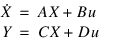
In all cases, all computed eigenvalues may be expressed as:
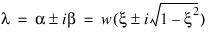 | (30) |
Where w is defined as the undamped natural frequency and  is defined as the damping ratio. Solving Equation (30) for both the undamped natural frequency and the damping ratio, we get the following results for real-only eigenvalues:
is defined as the damping ratio. Solving Equation (30) for both the undamped natural frequency and the damping ratio, we get the following results for real-only eigenvalues: | (31) |
For complex eigenvalues Equation (30) results in:
 | (32) |
See Eigenvalue Table Reported in Adams View for an example output showing the computed undamped natural frequency, damping ratio, real value and imaginary value of the displayed eigenvalues of the model.
Table 1 Eigenvalue Table Reported in Adams View
Mode Number | Undamped Natural Frequency  | Damping Ratio  | Real  | Imaginary  |
|---|---|---|---|---|
1 | 0.00617426 | 1 | -0.00617426 | 0 |
2 | 16.6257 | 1 | -16.6257 | 0 |
3 | 0.270866 | 0.23569 | -0.0638404 | +/-0.263235 |
4 | 0.712246 | 0.580427 | -0.413406 | +/-0.57999 |
Eigenvalues can be plotted as a complex scatter on a real-imaginary axis, as shown in Figure 1 Complex Scatter Plot. The real part of eigenvalues corresponds to damping in a model. The imaginary part corresponds to stiffness in the model. A mode with an eigenvalue of negative real part is considered stable. Conversely, a mode with eigenvalues of positive real part is unstable. As shown in Figure 1 Complex Scatter Plot, eigenvalues lying in the left half plane are stable and those in the right half plane are unstable.

Figure 1 Complex Scatter Plot
A model with all stable eigenvalues, if perturbed, will return to its original unperturbed configuration on removal of the perturbation. A perturbation applied to a model with unstable eigenvalue(s) may cause unstable modes to be excited. In this case, the model will have an unbounded response to this perturbation. For more information, see Reference 4.
Regarding computed mode shapes  , Adams Vibration does not export the computed mode shapes. Should you need the computed raw mode shapes from matrix A, we suggest exporting the A matrix and compute the mode shapes using an eigensolver of your choice. The A may be exported using the LINEAR/STATEMAT Solver command or using the Adams View user interface.
, Adams Vibration does not export the computed mode shapes. Should you need the computed raw mode shapes from matrix A, we suggest exporting the A matrix and compute the mode shapes using an eigensolver of your choice. The A may be exported using the LINEAR/STATEMAT Solver command or using the Adams View user interface.For animation purposes, Adams Vibration uses the following equation:
 | (33) |
to obtain all coordinates in the model for given a particular mode shape. Matrix T is a transformation matrix from the minimal state-space representation to the full representation of the model. Vector Q is used to animate the mode shapes in the post processor and to display the Normalized Coordinates in the Energy Tables options. A similar transformation is used to compute the velocity and differential states allowing the computation of Kinetic Energy, Strain Energy and Dissipative Energy tables.
Forced Vibration Analysis
Forced vibration analysis, forced response analysis, and frequency response analysis are synonyms in this context. A forced response analysis (FRA) in Adams Vibration requires you to create sets of input channels (u) and output channels (Y) as described in the Building Your Model section.
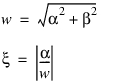
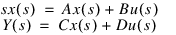
The FRA begins by first building the state-space representation:
 | (34) |
As shown in the previous section, vector X stands for the minimal state-space representation, matrix A is the linearization matrix and matrices B, C and D are the input/output matrices computed using the definitions of the input and output channels. Adams Vibration requires you to construct a vibration analysis using the graphical interface. A vibration analysis consists of a collection of all the input and output channels, the operating point specification, the frequency range and number of steps in this range. Options to turn off damping matrices and the usage of user-defined states are also available.
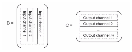
Figure 2 Input and Output Channels
When using the Adams Vibration user interface to create an input channel, each input channel results in an action-only SFORCE being created in the model along with a VARIABLE. The VARIABLE is used to define the SFORCE. The expression for the variable is set to zero in the Adams Solver model because the computation of the B and D matrices do not require a value for the said VARIABLE. However, the input channel definition will be used in the FRA subsequent analysis.
When creating an output channel, each output channel results in one VARIABLE being created. Function expression for this entity depends on the type of output channel you define. On defining a vibration analysis, the variable corresponding to the input channels are collected into a PINPUT and variables corresponding to the output channels are collected into a POUTPUT. The model is linearized using this PINPUT and POUTPUT pair. As shown in Figure 2. Input and Output Channels, each input channels contributes one column to the B matrix. Each output channel defines one row of the C matrix.
The FRA proceeds with taking the Laplace transform of Equation (34) to obtain:
 | (35) |
Where s is the Laplace variable and x(s), u(s) and Y(s) are the transforms of X, u and Y respectively. Solving for Y(s) we find:
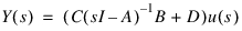 | (36) |
Defining the transfer function H(s) as:
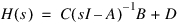 | (37) |
The forced response of all output channel is then:
 | (38) |
Adams Vibration will compute the value of each Y(s) for each s specified in the Vibration Analysis definition.
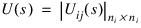
If the size of vector X is N, and there are ni inputs and there are no outputs, then the sizes of the matrices in Equation (37) are:
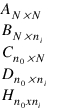
Adams Vibration user interface allows the user to set a range of values for the variable s using different formats. Notice that for each s computing the response Y(s) requires inverting a matrix of size NxN as shown in Equation (37). If matrix A can be diagonalized, the response for each s is obtained following the diagonalization algorithm shown in section Transformation to Modal Space.
Transfer Function
The plots for the transfer function H(s) are computed from equation (37). Adams Post Processor displays each plot by first selecting an input channel k and then selecting an output channel j in the post-processing window. Each plot corresponds to the entry Hjk of the H(s) matrix for all values of s.
These plots are equivalent to setting input channel k to 1 and all other input channels to zero in Equation (38), and displaying the jth entry of the resulting matrix-vector multiplication. See Figure 3 below.
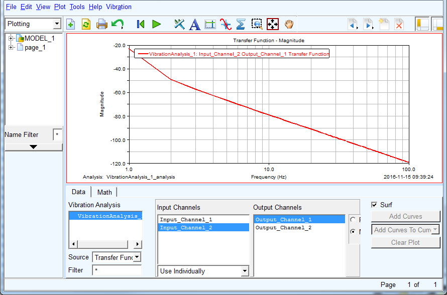
Figure 3 Transfer Function plots.
Besides displaying each entry of the transfer function matrix H(s), Adams Post Processor allows plotting the frequency response Y(s) for each output channel. Equation (38) may be rewritten as follows:
 | (39) |
The post processor plots each individual contribution of each input channel Hkj(s) uj(s) or the total sum. The computed value is, in general, a complex value. The plots are computed for:

Here sb and se are the Begin and End frequencies respectively as set by the user in the Vibration Analysis user interface.
PSD Response Computation
Equation (39) provides the standard frequency response of the system's outputs given a set of inputs in the frequency domain. However, in the field of Random Vibrations, analysts have the Power Spectral Density Sxx(s) of an input and the objective is to compute the Power Spectral Density Syy(s) of an output. In this case, the relation between a single PSD input Sxx(s) and a single PSD output Syy(s) with transfer function h(s) is:
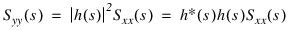
Where h*(s) stands for the complex conjugate of h(s).
Adams Vibration can be used to define input channels with actuators of either PSD type or non-PSD type. Actuators of the non-PSD type are standard actuators with computed Fourier Transforms obtained from measured input signals or theoretical functions entered as symbolic expressions in the user interface. Actuators of the PSD type define a Power Spectral Density function (the Fourier Transform of the autocorrelation of some signal).
Regardless of the type of input channels (either PSD type or non-PSD type), Adams Vibration computes and displays the Power Spectral Density response of each output channel, or PSD(s).
For input channels using non-PSD type actuators, a non-standard estimation of the Power Spectral Density is computed as follows:
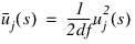 | (40) |
Here df is the difference between End and Begin frequencies as setup in the Vibration Analysis data. Notice this estimation of the Power Spectral Density returns complex values. Using Equation (40), the response PSD(s) is computed using the standard equation:
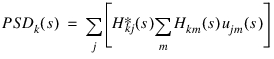
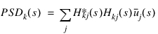 | (41) |
Here PSDk(s) is the response Power Spectral Density function for the kth output. Hkj*(s) is the complex conjugate of Hkj(s). The summation is implied 1 to ni. Adams Post Processor does not compute the individual contribution of each input channel when displaying PSDk(s). Notice we assume there are no cross correlations between the inputs.
For actuators of the PSD type there are two cases to consider. If there are no cross-power spectral actuators between the different input channels, the PSD(s) output is computed using the standard equation:
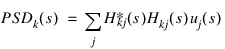 | (42) |
If there is a set of cross-power spectral actuators U(s), they can be ordered in matrix form as:
 | (43) |
For this second case, the Power Spectral Density response PSD(s) is computed as:
 | (44) |
Adams Vibration user interface provides the tools to define the matrix of cross-spectral actuators. When defining a PSD type input channel Uii(s), check the Cross Correlation checkbox and click the Cross Correlation Setup button to define the cross-spectral actuators Uij(s).
When plotting PSD response, input channels with actuators of type PSD cannot be mixed with actuators of force type in one vibration analysis.
Units of SPLINE data for PSD input data
When defining PSD input data for force input channel by using SPLINE elements, the units of the SPLINE data must be given in:
(force units)2/(frequency units)
where force units and frequency units match the global units set in the Adams model. In other words, the units of the PSD data must be consistent with the units of the model. Once the Adams Vibration analysis is completed, the output signals will have consistent units as specified in the system units for the model. Similarly, if the input channel is an acceleration input channel, then the units of a PSD actuator must be given in:
(acceleration units)2/(frequency units)
Modal Coordinates
Equation (35) can be transformed from the standard state-space representation into a "modal" representation. We define the "modal" states q(t) as follows:
 | (45) |
Matrix Z in Equation (45) is the modal matrix composed by the mode shapes obtained from the eigensolution of the system. Notice Equation (45) is a representation of the solution x(t) in the time domain. Transforming Equation (45) into the frequency domain, we obtain:
 | (46) |
Using Equation (46) into Equation (35) and simplifying we obtain an equivalent representation of the frequency response of the system in terms of the "modal" states q(s):
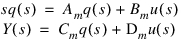 | (47) |
Matrices Am, Bm, and Cm are obtained from:
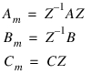 | (48) |
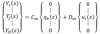
Adams Vibration computes and displays the frequency response of each modal state qk(s). From Equation (47) we obtain in matrix form:
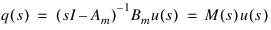 | (49) |
Equation (49) can be interpreted as the frequency response of each modal state. Moreover, for a given input channel j and a given entry k in the modal vector q(s), Adams Vibration computes and plots:
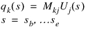 | (50) |
Equation (50) is the frequency response of the kth entry in the modal vector due to the jth input channel. Adams Post Processor displays Equation (50) for the complete range of selected frequencies s. See Figure 4 below.
Note: | Currently, in the Modal Coordinates plot options, the user interface wrongly shows the number of different eigenvalues instead of the size of the state vector q(s). The modification of the user interface will be executed in compliance with enhancement ADMS-37553. |
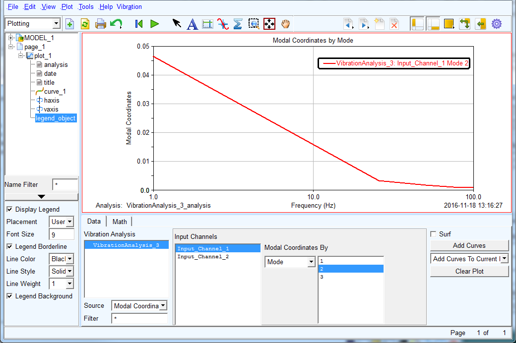
Figure 4 State space frequency response
While Equation (50) displays the response of a single state qk(s) for the whole range of specified frequencies s, Adams Post Processor also displays the complete response of the modal vector q(s) for a given frequency so. Evaluating Equation (49) for s=so and for the jth input channel (all other input channels are set to zero) we obtain:
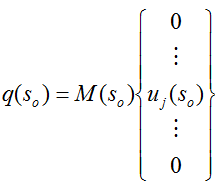 | (51) |
Vector q(so) is of size N (which is the size of the state matrix A) and Adams Post Processor display the contents of this array.
See Figure 5 for an example plot of Equation (51). Notice the horizontal axis is the mode number from 1 to N where N is the size of the linearization matrix A (see Equation (25)).
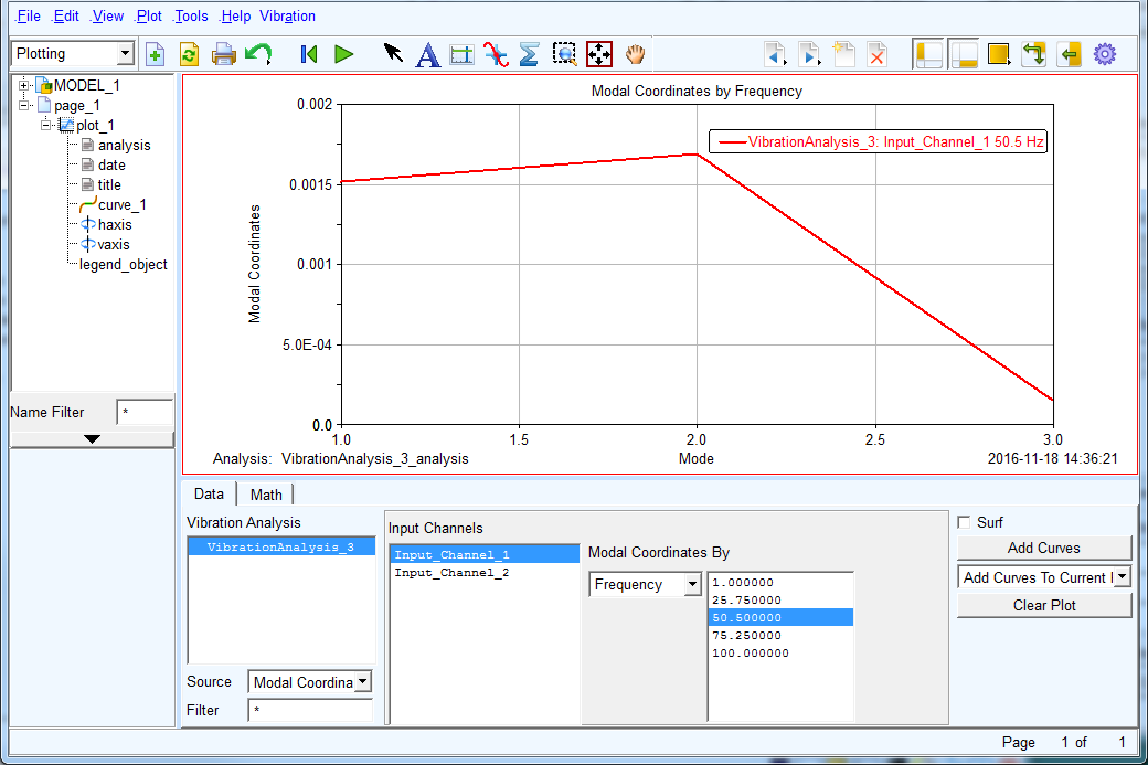
Figure 5 State vector for a given frequency and input.
Modal Participation
While the modal coordinates define how active a certain mode qk(s) is at a given frequency s (see Equation (50)), the modal participation identifies how much a given input ui(s) and a given mode qk(s) contribute to the total frequency response of a specified output Yj(s). From Equation (47) we obtain:
 | (52) |
The options to plot the Modal Participation in the Adams Post Processor allow selecting the ith input, the kth mode and the jth output. See Figure 6 below.
Note: | Currently the plotting options, in Modal Participation plot, wrongly show the number of different eigenvalues instead of the full range of modal coordinates. Also there is an incorrect algorithm implementation providing approximate results only. The user interface and implemented algorithm will be corrected following enhancement ADMS-37565. |
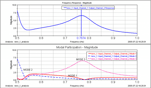
Figure 6 Plot of Modal Participations
Modal Energy Computation
In addition to showing modal coordinates tables, the user interface may show modal energy tables (kinetic, strain and dissipative) for each computed eigenvalue/eigenvector pair. Given that the computations are done using normalized eigenvectors, the units of length have been dropped out. For example, reported kinetic energy will be reported with units of User-mass/time^2 instead of units of User-mass * length^2/time^2.
i. Kinetic energy distribution – Mass bearing modeling objects such as PART, POINT_MASS, and FLEX_BODY contribute to kinetic energy distribution computation. The modal kinetic energy distribution in a system is defined with respect to degree of freedom of various modeling elements mentioned above.
The modal kinetic energy of ith mode can be calculated as
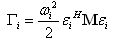 | (53) |
where:
 i
i■ = System mass matrix
= System mass matrixTo find modal energy contributions from various parts and degrees of freedom, it is convenient to substructure this system level energy equation to part level equations. Finally, these sub-structured part level energies will be summed to calculate the system level modal kinetic energy.
Kinetic energy contribution of PART j to individual mode i can therefore be written as,
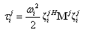 | (54) |
where:
■ ith column vector corresponding to six degrees of freedom of PART j. This vector is a subset of column mode shape vector.
ith column vector corresponding to six degrees of freedom of PART j. This vector is a subset of column mode shape vector. ■ = Mass matrix of PART j
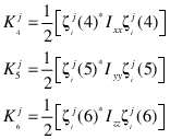
= Mass matrix of PART jAdams Vibration breaks this modal kinetic energy contribution of PART j in nine components to present it in modal energy tables:
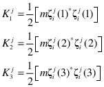 | (55) |
Equation (54) now equivalently expressed as,
 | (56) |
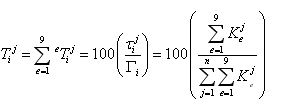
Total kinetic energy for mode i can then be computed as,
 | (57) |
where:
■ = Total kinetic energy of mode i
= Total kinetic energy of mode i■n = Number of parts in the model
■ Kinetic energy contribution of PART j to mode i
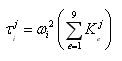
Kinetic energy contribution of PART j to mode iPercentage distribution of PART j mode i kinetic energy in direction e is defined as:
 | (58) |
Above equation shows that the percentage kinetic energy contribution of any degree of freedom to a particular mode is independent on natural frequency of that mode and depends on the product of the mass or inertia and square of the mode shape amplitude (mass and inertia terms) or product of mode shape amplitudes (product of inertia terms) of the mode in that directions. As the sum of the kinetic energy contributions of all degree of freedoms in that mode shape (not part degrees of freedom) is made equal to 100, through the definition in Equation (58), it is easy to identify the relative importance of various degrees of freedoms. This will help to identify which particular degree of freedom is contributing more or less to the overall modal kinetic energy.
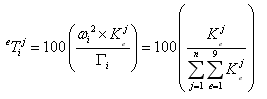
Percentage kinetic energy contributed by PART j to mode i is defined as:
 | (59) |
where:
■ = Percentage kinetic energy contributed by PART j to mode i
= Percentage kinetic energy contributed by PART j to mode iEquation (59) shows that the percentage kinetic energy contribution of any part to a particular mode is independent on natural frequency of that mode and depends on the sum of product of mass (or inertia) and square of the mode shape amplitude (mass and inertia terms) or product of mode shape amplitudes (product of inertia terms) of that mode in all nine directions. As the sum of the kinetic energy contributions of all parts is made equal to 100, it is easy to identify the relative importance of various parts over each other. This will help to identify which particular part of model is contributing more or less to the overall modal kinetic energy.
It should be noted that the large kinetic energy contribution can be due to large mass (inertia) or motion of that degree of freedom. Therefore, the modal kinetic energy density needs to be calculated to remove this ambiguity and make it dependent only on mode shape. The modal kinetic energy density for a given mode is defined as the ratio of modal kinetic energy contribution of a degree of freedom to the rigid body mass of the part.
Sometimes it is advantageous to normalize the modal kinetic energy contributions with respect to generalized mass of that mode. This will make these modal kinetic energy distributions independent of mode shape normalization.
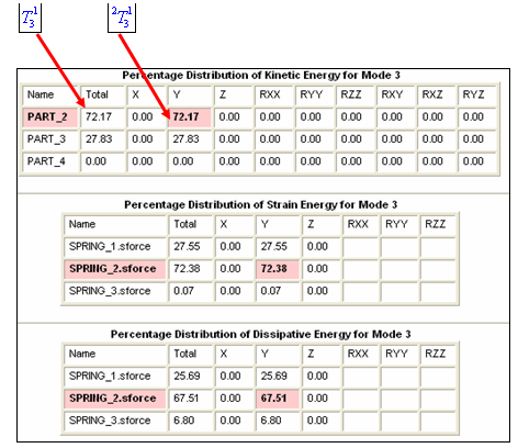
Adams Vibration computes the kinetic, strain, and dissipative energy distribution within modes of your model. Table 1 Modal Energy Distribution shows an example of these distribution tables. These distributions are important indicators of which components of the model have the greatest contribution to a given mode.
As in this example, PART_2 has the greatest contribution to the kinetic energy in this mode. The Strain energy tables indicate that SPRING_2 stores the most amount of strain energy in this mode. Similarly, from the dissipative energy table, SPRING_2 dissipates the most amount of energy in this mode.
Table 1 Modal Energy Distribution
ii. Strain energy distribution - Compliant components, such as SPRINGDAMPER, SFORCE, BUSHING, and so on, contribute to the computation of strain energy in a mode. In addition, FLEX_BODYs in the model contribute to strain energy computation.
Strain energy due to a compliant element p is:
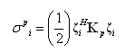 | (60) |
where:
■ = Strain energy in complaint element p for mode i
= Strain energy in complaint element p for mode i■ = Matrix of size equal to model stiffness matrix, with all zero entries except stiffness matrix entries contributed by compliant element p.
= Matrix of size equal to model stiffness matrix, with all zero entries except stiffness matrix entries contributed by compliant element p. Percentage distribution of strain energy for mode i is given as:
 | (61) |
where:
■ = Percentage strain energy contribution by compliant element p to mode i
= Percentage strain energy contribution by compliant element p to mode i■m = Number of compliant elements in the model
iii. Dissipative energy distribution is computed in a similar manner to the strain energy distribution. In equation (60)  ; p, the damping matrix is substituted for the stiffness matrix.
; p, the damping matrix is substituted for the stiffness matrix. Stress Recovery
With Adams Vibration you can recover stresses and strains on flexible bodies. Recovering stresses on flexible bodies is called Modal Stress Recovery (MSR). Adams Vibration allows you to export modal-coordinates corresponding to flexible body modes that can later be used as input to FEM software like Nastran to recover the stresses in the flexbody.
The linear deformation (y) of the flexbody nodes can be approximated as a linear combination of M orthogonalized mode shape vectors ( ) of that flexbody.
) of that flexbody. 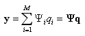 | (62) |
The basic advantage of the modal superposition is that the deformation behavior of a component with a very large number of nodal DOF can be captured with a much smaller number of modal DOF.
Adams Vibration exports the modal coordinates ( ) in a Modal Deformation File (MDF) format (binary). FEM software like Nastran then does the summation to get linear deformation of flexbody nodes and then recovers stresses and strains as follows,
) in a Modal Deformation File (MDF) format (binary). FEM software like Nastran then does the summation to get linear deformation of flexbody nodes and then recovers stresses and strains as follows,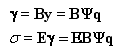 | (63) |
where:
■ is the strain vector
is the strain vector■ is the stress vector
is the stress vector■B is a function matrix of the FE geometry relating strains to displacements
■E is the stress-strain relationship matrix.
Note that it is necessary to create a super-element of flexbody without any constraints (free-free boundary condition). The restart run is necessary in Nastran to recover the stresses and strains.