Adams Basic Package > Adams View > Adams View > Dialog box - F1 help > A - D > Create/Modify Contact

Create/Modify Contact

Ribbon menu → Forces Tab -→ Special Forces Container → Create/Modify Contact

Creates or modifies a contact force between two geometries. Learn About Contact Forces. For solids and curves, you can select more than one geometry as long as the geometry belongs to the same part. The first geometry is called the I geometry and the second geometry is called the J geometry. For sphere-to-sphere contacts, you can specify that the contact be inside or outside the sphere.

Learn more about Contacts.

For the option:	Do the following:
Tips on Entering Object Names in Text Boxes. If you type a geometry object name directly in the text box, you must press Enter to register the value.
Contact Name	Enter the name of the contact to create or modify.
Contact Type	Set to the type of geometry to come into contact. The text boxes change depending on the type of contact force you selected.
If you selected Solid to Solid, Adams View displays the following two options:
I Solid	Enter one or more geometry solids. The solids must all belong to the same part.
J Solid	Enter one or more geometry solids. The solids must all belong to the same part.
If you selected Curve to Curve, Adams View displays the following four options:
I Curve	Enter one or more geometry curves. The curves must all belong to the same part.
I Direction(s)	Select the geometry on which you want to change the direction of the force, and then select the Change Direction tool .
J Curve	Enter one or more geometry curves. The curves must all belong to the same part.
J Direction(s)	Select the geometry on which you want to change the direction of the force, and then select the Change Direction tool .
If you selected Point to Curve, Adams View displays the following two options:
Marker	Enter a marker.
Curve	Enter one or more curves.
Direction(s)	Select the geometry on which you want to change the direction of the force, and then select the Change Direction tool .
If you selected Point to Plane, Adams View displays the following two options:
Marker	Enter a marker.
Plane	Enter a plane.
If you selected Curve to Plane, Adams View displays the following two options:
Curve	Enter one or more curves.
Direction(s)	Select the geometry on which you want to change the direction of the force, and then select the Change Direction tool .
Plane	Enter a plane.
If you selected Sphere to Plane, Adams View displays the following two options:
Sphere	Enter a sphere. To change the direction of the force, select the Change Direction tool .
Direction(s)	Select the geometry on which you want to change the direction of the force, and then select the Change Direction tool .
Plane	Enter a plane.
If you selected Sphere to Sphere, Adams View displays the following two options: Note: If the internal surface(s) of one geometry is selected to be used for contact via the Change Direction tool, then the other geometry should be contained or nearly contained by the other's surface(s) in the model design position otherwise the contact force will return a very large value initially.
Sphere	Enter a sphere. To change the direction of the force, select the Change Direction tool .
Sphere	Enter a sphere. To change the direction of the force, select the Change Direction tool .
If you selected Cylinder to Cylinder, Adams View displays the following three options: Note: If the internal surface(s) of one geometry is selected to be used for contact via the Change Direction tool, then the other geometry should be contained or nearly contained by the other's surface(s) in the model design position otherwise the contact force will return a very large value initially.
First Cylinder	Enter a cylinder. To change the direction of the force, select the Change Direction tool .
Second Cylinder	Enter a cylinder. To change the direction of the force, select the Change Direction tool .
Face Contact	For cylinder-in-cylinder scenarios (that is, where the interior surface of one of the cylinders was selected) the faces of the outer cylinder can be optionally set to enforce contact. The “Bottom” face is defined as the one on which the cylinder geometry’s reference marker is located. The "Top" face is defined as the one on which the cylinder geometry's reference marker is NOT located.
If you selected Flex Body to Solid, Adams View displays the following two options:
I Flexible Body	Select a Flexible Body.
J Solid	Select a Geometry Solid.
If you selected Flex Body to Flex Body, Adams View displays the following two options:
I Flexible Body	Select a Flexible Body.
J Flexible Body	Select a Flexible Body.
If you selected Flex Edge to Curve, Adams View displays the following three options:
I Flexible Body	Select a Flexible Body. To reset the Edge, select the Reset The Edge tool .
I Flex Edge	Select a Flex Edge on I Flexible Body. To change the direction of the force, select the Change Direction tool .
J Curve	Select a Curve. Multiple curves are not allowed.
If you selected Flex Edge to Flex Edge, Adams View displays the following four options:
I Flexible Body	Select a Flexible Body. To reset the Edge, select the Reset The Edge tool .
I Flex Edge	Select a Flex Edge on I Flexible Body. To change the direction of the force, select the Change Direction tool .
J Flexible Body	Select a Flexible Body. To reset the Edge, select the Reset The Edge tool .
J Flex Edge	Select a Flex Edge on J Flexible Body. To change the direction of the force, select the Change Direction tool .
If you selected Flex Edge to Plane, Adams View displays the following three options:
I Flexible Body	Select a Flexible Body. To reset the Edge, select the Reset The Edge tool .
I Flex Edge	Select a Flex Edge on I Flexible Body. To change the direction of the force, select the Change Direction tool .
Plane	Select a Plane. Multiple Planes are not allowed.
The following options apply to all types of geometry:
Force Display/Color	Select to turn on the force display of both normal and friction forces, and select a color for the force display. Note: If you are using an External Adams Solver, you must set the output files to XML to view the force display. See Solver Settings - Output dialog box help.
Normal Force	Select either: ■Restitution - To define the normal force as restitution-based. This option is not available with Flex Body to Solid and Flex Body to Flex Body type of contacts. ■Impact - To define the normal force based on an impact using the IMPACT function. ■User Defined - To define the force based on a User-written subroutine. Learn about the types of Contact Force Algorithms and also see Learning More about the Contact Detection Algorithm.
If you selected Restitution for Normal Force, define the following two options:
Penalty	Enter a penalty value to define the local stiffness properties between the contacting material. A large penalty value ensures that the penetration of one geometry into another will be small. Large values, however, will cause numerical integration difficulties. A value of 1E6 is appropriate for systems modeled in Kg-mm-sec. For more information on how to specify this value, see the Extended Definition for the CONTACT statement in the Adams Solver online help. Note: The penalty value of 1.0E+06 is recommended value for users who have no prior experience with restitution based contacts. Experienced users will find values that are both smaller and larger that are applicable to their models. The value of 1.0E+06 was determined heuristically by simulating real world models (for example, billiard ball collisions). It is appropriate for bodies with masses in the range of 0.1 to 1.0e+03 Kilograms and velocities in the range of 0.01 to 1.0e+03 meters/second. For collisions involving asteroids, a larger value may be needed. Many contact parameters (for example, stiffness, damping, exponent) have default values that are not suitable for all models. They are intended to help users who has very little modeling background. The reason that contact parameters exist is to give users as much flexibility as possible in building and simulating their models.
Restitution Coefficient	Enter the coefficient of restitution, which models the energy loss during contact. ■A value of zero specifies a perfectly plastic contact between the two colliding bodies. ■A value of one specifies a perfectly elastic contact. There is no energy loss. The coefficient of restitution is a function of the two materials that are coming into contact. For information on material types versus commonly used values of the coefficient of restitution, see the table for the CONTACT statement in the Adams Solver online help.
If you selected Impact for Normal Force, define the following four options:
Stiffness	Enter a material stiffness that is to be used to calculate the normal force for the impact model. In general, the higher the stiffness, the more rigid or hard the bodies in contact are. Note: When changing the length units in Adams View, stiffnesses in contacts are scaled by (length conversion factor**exponent). When changing the force unit, stiffness is only scaled by the force conversion factor.
Force Exponent	Adams Solver models normal force as a nonlinear springdamper. If the damping penetration, below, is the instantaneous penetration between the contacting geometry, Adams Solver calculates the contribution of the material stiffness to the instantaneous normal forces as: STIFFNESS * (PENALTY)**EXPONENT For more information, see the IMPACT function in the Adams Solver online help.
Damping	Enter a value to define the damping properties of the contacting material. Consider a damping coefficient that is about one percent of the stiffness coefficient.
Penetration Depth	Enter a value to define the penetration at which Adams Solver turns on full damping. Adams Solver uses a cubic STEP function to increase the damping coefficient from zero, at zero penetration, to full damping when the penetration reaches the damping penetration. A reasonable value for this parameter is 0.01 mm. For more information, see the IMPACT function in the Adams Solver online help.
If you selected User Defined for Normal Force, define the following two options:
User function	Specify the user parameters to be passed to a User-written subroutine CNFSUB. For more on user-written subroutines, see the Adams Solver online help.
Routine	Specify an alternative library and name for the user subroutine. Learn about ROUTINE Argument.
The following option is available for all choices:
Augmented Lagrangian	Select to refine the normal force between two sets of rigid geometries that are in contact. When you select Augmented Lagrangian, Adams View uses iterative refinement to ensure that penetration between the geometries is minimal. It also ensures that the normal force magnitude is relatively insensitive to the penalty or stiffness used to model the local material compliance effects. Note: Augmented Lagrangian is only available when defining a Restitution-based contact. It is only used when running the Adams Solver Fortran executable. Adams Solver C++ ignores this selection.
Friction Force	Select to model the friction effects at the contact locations using the Coulomb friction model, Stiction and Sliding, no friction, or as user-defined subroutine. The Coulomb friction model models dynamic friction but not stiction in contacts. For more on friction in contacts, see Contact Friction Force Calculation. In addition, read the information for the CONTACT statement in the Adams Solver online help.
If you selected Coulomb for Friction Force, define the following four options:
Coulomb Friction	Specify whether the friction effects are to be included at run time: ■On ■Off ■Dynamics Only
Static Coefficient	Specify the coefficient of friction at a contact point when the slip velocity is smaller than the value for Static Transition Vel. For information on material types versus commonly used values of the coefficient of static friction, see Material Contact Properties Table. Excessively large values of Static Coefficient can cause integration difficulties. Range: Static Coefficient 0
Dynamic Coefficient	Specify the coefficient of friction at a contact point when the slip velocity is larger than the value for Friction Transition Vel. For information on material types versus commonly used values of the dynamic coefficient of friction, see Material Contact Properties Table. Excessively large values of Dynamic Coefficient can cause integration difficulties. Range: 0 Dynamic Coefficient Static Coefficient
Stiction Transition Vel.	Enter the static transition velocity. The figure below shows how the coefficient of friction varies with slip velocity at a typical contact point. 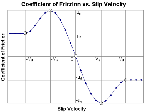In this simple model: ■ ■ ■ ■ ■ ■ ■(v) = -step(\|v\|,vs,s, vd, d) sign(v) for vs < \|v\| < vd ■
Stiction Transition Vel. (cont.)	In the figure: ■Vs, the slip velocity at which the coefficient friction achieves a maximum value of , is denoted as STICTION_TRANSITION_VELOCITY. ■ is the coefficient of static friction. ■ is the coefficient of dynamic friction. For more on friction in contacts, see Contact Friction Force Calculation. In addition, read the information for the CONTACT statement in the Adams Solver online help. Range: 0 < Stiction Transition Vel. Friction Transition Vel.
Friction Transition Vel.	Enter the friction transition velocity. Adams Solver gradually transitions the coefficient of friction from the value for Static Coefficent to the value for Dynamic Coefficient as the slip velocity at the contact point increases. When the slip velocity is equal to the value specified for Friction Transition Vel., the effective coefficient of friction is set to Dynamic Coefficient. For more on friction in contacts, see Contact Friction Force Calculation. In addition, read the information for the CONTACT statement in the Adams Solver online help. Note: Small values for this option cause the integrator difficulties. You should specify this value as: Friction Transition Vel. 5* ERROR where: ERROR is the integration error used for the solution. Its default value is 1E-3. Range: Friction Transition Vel. Static Transition Vel. > 0
If you selected Stiction and Sliding for Friction Force, define the following Six options:
Friction mode	Specify whether the friction effects are to be included at run time: ■On ■Dynamics Only
Static Coefficient	Specify the coefficient of friction at a contact point when the slip velocity is smaller than the value for Static Transition Vel. For information on material types versus commonly used values of the coefficient of static friction, see Material Contact Properties Table. Excessively large values of Static Coefficient can cause integration difficulties. Range: Static Coefficient 0
Dynamic Coefficient	Specify the coefficient of friction at a contact point when the slip velocity is larger than the value for Friction Transition Vel. For information on material types versus commonly used values of the dynamic coefficient of friction, see Material Contact Properties Table. Excessively large values of Dynamic Coefficient can cause integration difficulties. Range: 0 Dynamic Coefficient Static Coefficient
Stiction Transition Vel.	Enter the static transition velocity. The figure below shows how the coefficient of friction varies with slip velocity at a typical contact point. In this simple model: ■ ■ ■ ■ ■ ■ ■(v) = -step(\|v\|,vs,s, vd, d) sign(v) for vs < \|v\| < vd ■
Stiction Transition Vel. (cont.)	In the figure: ■Vs, the slip velocity at which the coefficient friction achieves a maximum value of , is denoted as STICTION_TRANSITION_VELOCITY. ■ is the coefficient of static friction. ■ is the coefficient of dynamic friction. For more on friction in contacts, see Contact Friction Force Calculation. In addition, read the information for the CONTACT statement in the Adams Solver online help. Range: 0 < Stiction Transition Vel. Friction Transition Vel.
Friction Transition Vel.	Enter the friction transition velocity. Adams Solver gradually transitions the coefficient of friction from the value for Static Coefficent to the value for Dynamic Coefficient as the slip velocity at the contact point increases. When the slip velocity is equal to the value specified for Friction Transition Vel., the effective coefficient of friction is set to Dynamic Coefficient. For more on friction in contacts, see Contact Friction Force Calculation. In addition, read the information for the CONTACT statement in the Adams Solver online help. Note: Small values for this option cause the integrator difficulties. You should specify this value as: Friction Transition Vel. 5* ERROR where: ERROR is the integration error used for the solution. Its default value is 1E-3. Range: Friction Transition Vel. Static Transition Vel. > 0
Max Stiction Deformation	Define the maximum displacement that can occur in a contact once the frictional force in the contact enters the stiction regime. The slight deformation allows Adams Solver to easily impose the Coulomb conditions for stiction or static friction, for example: Friction force magnitude < static * normal force Therefore, even at zero velocity, you can apply a finite stiction force if your system dynamics require it. The default is 0.01 length units, and the range is > 0.
If you selected User Defined for Friction Force, define the following two options:
User function	Specify the user parameters to be passed to a user-written subroutine. For more on user-written subroutines, see Adams Solver online help.
Routine	Enter the name of the function to call. The default is CNFSUB.