CONTACT
The CONTACT statement lets you define a two- or three-dimensional contact between a pair of geometric objects. Adams Solver (C++) models the contact as a unilateral constraint, that is, as a force that has zero value when no penetration exists between the specified geometries, and a force that has a positive value when penetration exists between two geometries.
The CONTACT statement supports:
■Multiple contacts
■Dynamic friction
■Stiction
■Contact between three-dimensional solid geometries
■Contact between two-dimensional geometries
It does not support non-solid three-dimensional geometries, such as shells that do not encompass a volume and sheets. It also does not support contact between a two-dimensional and a three-dimensional geometry.
Adams Solver (C++) has two geometry engines that it uses for three-dimensional contacts. It uses Parasolid, a geometry toolkit from EDS/Unigraphics, and RAPID. Currently, RAPID is the default and Adams Solver (C++) supports version 2.01.
Adams Solver understands some geometries as analytical. Whenever possible use analytical geometries to speed up solution time and realize smoother contact forces. Analytical geometries are created via the GRAPHICS/ statement. The table further below illustrates which geometry types Adams Solver treats analytically.
Note that the tessellation of a box is simple enough (12 triangles) such that it performs as well as an analytical box would.
For two-dimensional contacts, Adams Solver (C++) uses an internally developed geometry engine. Currently, Adams Solver (C++) supports Parasolid version 35. See the Extended Definition for more information.
The geometry engine is responsible for detecting contact between two geometries, locating the points of contact, and calculating the common normal at the contact points.
Once the contact kinematics are known, contact forces, which are a function of the contact kinematics, are applied to the intersecting bodies.
Note: | You can only define two-dimensional contacts between bodies that are constrained to be in the same plane. This is usually done with planar or revolute joints or an equivalent set of constraints that enforce the planarity. Failure to enforce planarity will result in a run-time error, when the bodies go out of plane during a simulation. |
The following table shows the legal combinations of geometry for the CONTACT statement. If you use unsupported geometry combinations, you will receive an error.
Supported Geometry Combinations
Note: | You can set the default geometry library. See the PREFERENCES statement. |
Format
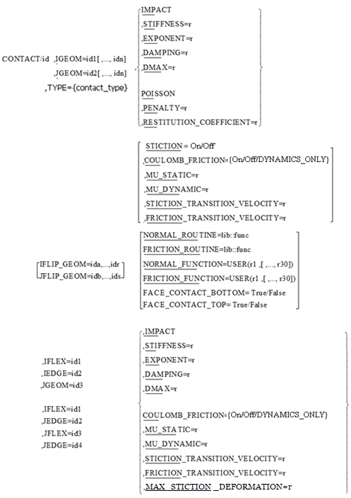
Arguments
COULOMB_FRICTION = off/on/DYNAMICS_ONLY | Models friction effects at the contact locations using the Coulomb friction model to compute the frictional forces. ■The friction model in CONTACT models dynamic friction but not stiction. ■The argument values, On/Off/DYNAMICS_ONLY, specify at run time whether the friction effects are to be included. If the value is On, the friction is active in all simulation types. If the value is Off, the friction is deactivated in all simulation types. If the value is DYNAMICS_ONLY, the friction is active only during dynamic simulations. |
DAMPING = r | Used when you specify the IMPACT model for calculating normal forces. DAMPING defines the damping properties of the contacting material. You should set the damping coefficient is about one percent of the stiffness coefficient. Range: DAMPING >0 |
DMAX = r | Used when you specify the IMPACT model for calculating normal forces. DMAX defines the penetration at which Adams Solver turns on full damping. Adams Solver uses a cubic STEP function to increase the damping coefficient from zero, at zero penetration, to full damping when the penetration is DMAX. A reasonable value for this parameter is 0.01 mm. For more information, refer to the IMPACT function. Range: DMAX > 0 |
EXPONENT=r | Used when you specify the IMPACT model for calculating normal forces. Adams Solver (C++) models normal force as a nonlinear spring-damper. If PEN is the instantaneous penetration between the contacting geometry, Adams Solver calculates the contribution of the material stiffness to the instantaneous normal forces as STIFFNESS * (PENALTY)**EXPONENT. For more information, see the IMPACT function. Exponent should normally be set to 1.5 or higher. Range: 0 < EXPONENT |
FRICTION_TRANSITION_VELOCITY = r | Used in the COULOMB_FRICTION model for calculating frictional forces at the contact locations. Adams Solver (C++) gradually transitions the coefficient of friction from MU_STATIC to MU_DYNAMIC as the slip velocity at the contact point increases. When the slip velocity is equal to the value specified for FRICTION_TRANSITION_VELOCITY, the effective coefficient of friction is set to MU_DYNAMIC. For more details, see Extended Definition. Note: Small values for FRICTION_TRANSITION_VELOCITY cause the integrator difficulties. You should specify this value as: FRICTION_TRANSITION_VELOCITY > 5* ERROR where ERROR is the integration error used for the solution. Its default value is 1E-3. Range: FRICTION_TRANSITION_VELOCITY > STICTION_TRANSITION_VELOCITY > 0 |
FRICTION_FUNCTION=USER(r1[,...,r30]) | Specifies up to 30 user-defined constants to compute the contact friction force components in a user-defined subroutine, CFFSUB. |
FRICTION_ROUTINE = library::function | Specifies a library and a user-written subroutine in that library that calculates the contact friction force. |
IEDGE = id | ID of an edge on the IFLEX Body. Specifies a single edge. List of IDs is not supported. IEDGE cannot be used without IFLEX. IFLIP may be used with IEDGE. |
IGEOM = id | ID of the GRAPHICS statement that defines the first of two geometric bodies between which a CONTACT is to be modeled. Specifies a list of GRAPHICS IDs. The limit is 32,767. All geometries must belong to the same part. |
JGEOM = id | ID of the GRAPHICS statement that defines the second of two geometric bodies between which a CONTACT is to be modeled. Specifies a list of GRAPHICS IDs. The limit is 32,767. All geometries must belong to the same part. |
IFLEX = id | ID of the FLEX_BODY statement that defines the first of two flexible bodies between which a CONTACT is to be modeled. Specifies a single FLEX ID. List of IDs is not supported. |
JEDGE = id | ID of an edge on the JFLEX Body. Specifies a single edge. List of IDs is not supported. JEDGE cannot be used without JFLEX. JFLIP may be used with JEDGE. |
JFLEX = id | ID of the _BODY statement that defines the second of two flexible bodies between which a CONTACT is to be modeled. Specifies a single FLEX ID. List of IDs is not supported. |
IFLIP_GEOMETRY = id1,id2,...,idN | Specifies a list of GRAPHICS IDs associated with the IGEOM objects to be reversed in direction (flipped). Use IFLIP_GEOMETRY with two-dimensional geometries (for example, curves, arcs, and circles) and three-dimensional geometries (for example, cylinders and spheres as ellipsoids with equal axes). For an explanation of how CONTACT calculates tangents and normals, see Extended Definition. |
IMPACT | Specifies that the IMPACT method is to be used to model the normal force. For more information, see Extended Definition. |
JFLIP_GEOMETRY = id1,id2,...,idN | Specifies a list of GRAPHICS IDs associated with the JGEOM objects to be reversed in direction (flipped). Use JFLIP_GEOMETRY with two-dimensional geometries (for example, curves, arcs, and circles) and three-dimensional geometries (for example, cylinders and spheres as ellipsoids with equal axes). For an explanation of how CONTACT calculates tangents and normals, see Extended Definition. |
FACE_CONTACT_BOTTOM | Specific to cylinder-to-cylinder contacts where one of the cylinders is using its internal surface for contact (that is, referenced by I/JFLIP_GEOM). “Bottom” face is defined as the one on which the cylinder geometry’s reference marker is located. If set to “TRUE” then this face will enforce contact. |
FACE_CONTACT_TOP | Specific to cylinder-to-cylinder contacts where one of the cylinders is using its internal surface for contact (that is, referenced by I/JFLIP_GEOM). “Top” face is defined as the one on which the cylinder geometry’s reference marker is NOT located. If set to “TRUE” then this face will enforce contact. |
MAX_STICTION_DEFORMATION=r | Defines the maximum creep that can occur in a contact during the stiction regime. The creep allows Adams Solver (C++) to impose the Coulomb conditions for stiction or static friction, for example: Friction force magnitude <  * normal force * normal forceTherefore, even at zero velocity, a finite stiction force is applied if your system dynamics requires it. Default: 0.01 length units Range: MAX_STICTION_DEFORMATION > 0 |
MU_DYNAMIC = r | Specifies the coefficient of friction at a contact point when the slip velocity is larger than the FRICTION_TRANSITION_VELOCITY. For information on material types versus commonly used values of the coefficient of the dynamic coefficient of friction, see the Material Contact Properties table. Excessively large values of MU_DYNAMIC can cause integration difficulties. Range:0 < MU_DYNAMIC < MU_STATIC |
MU_STATIC=r | Specifies the coefficient of friction at a contact point when the slip velocity is smaller than the STICTION_TRANSITION_VELOCITY. For information on material types versus commonly used values of the coefficient of static friction, see the Material Contact Properties table. Excessively large values of MU_STATIC can cause integration difficulties. Range: MU_STATIC > 0 |
NORMAL_FUNCTION = USER(r1,[,...,r30]) | Specifies up to 30 user-defined constants to compute the contact normal force components in a user-defined subroutine, CNFSUB. |
NORMAL_ROUTINE = library::function | Specifies a library and a user-written subroutine in that library that calculates the contact normal force. |
PENALTY=r | Used when you specify a restitution model for calculating normal forces. PENALTY defines the local stiffness properties between the contacting material. A large value of PENALTY ensures that the penetration, of one geometry into another, will be small. Large values, however, will cause numerical integration difficulties. A value of 1E6 is appropriate for systems modeled in Kg-mm-sec. For more information on how to specify this value, see Extended Definition. Range: PENALTY > 0 |
POISSON | Specifies that a coefficient of restitution method is to be used to model the normal force. For more information, see the Extended Definition. |
RESTITUTION_COEFFICIENT = r | The coefficient of restitution models the energy loss during contact. A value of zero specifies a perfectly plastic contact between the two colliding bodies. A value of one specifies a perfectly elastic contact. There is no energy loss. The coefficient of restitution is a function of the two materials that are coming into contact. For information on material types versus commonly used values of the coefficient of restitution, the Material Contact Properties table. Range: 0 < RESTITUTION_COEFFICIENT < 1 |
STICTION = off/on | Models stiction effects at the contact locations using a stiction model similar to JOINT/FRICTION ■The stiction model in CONTACT models both stiction and dynamic friction. ■The argument values, On/Off, specify at run time whether the stiction effects are to be included. If the value is On, the stiction is active in all simulation types. If the value is Off, the stiction is deactivated in all simulation types. ■Stiction is available in contact Type = solid_to_solid and 3D analytical solid contact types i.e. cylinder_to_cylinder, sphere_to_sphere and sphere_to_plane. It is not available if other contact types are specified or if IMPACT argument is specified to model the normal force. |
STICTION_TRANSITION_VELOCITY = r | Used in the COULOMB_FRICTION model for calculating frictional forces at the contact locations. Adams Solver (C++) gradually transitions the coefficient of friction from MU_DYNAMIC to MU_STATIC as the slip velocity at the contact point decreases. When the slip velocity is equal to the value specified for STICTION_TRANSITION_VELOCITY, the effective coefficient of friction is set to MU_STATIC. For more details, see the Extended Definition. Note: A small value for STICTION_TRANSITION_VELOCITY causes numerical integrator difficulties. A general rule of thumb for specifying this value is: STICTION_TRANSITION_VELOCITY> 5 ERROR where ERROR is the accuracy requested of the integrator. Its default value is 1E-3. Range: 0 < STICTION_TRANSITION_VELOCITY < FRICTION_TRANSITION_VELOCITY |
STIFFNESS=r | Specifies a material stiffness that you can use to calculate the normal force for the impact model. In general, the higher the STIFFNESS, the more rigid or hard the bodies in contact are. Also note that the higher the STIFFNESS is, the harder it is for an integrator to solve through the contact event. |
TYPE = {contact_type} | Specifies contact type as: ■solid_to_solid ■curve_to_curve ■point_to_curve ■point_to_plane ■curve_to_plane ■sphere_to_plane ■sphere_to_sphere ■flex_to_solid ■flex_to_flex ■flex_edge_to_curve ■flex_edge_to_flex_edge ■flex_edge_to_plane ■cylinder_to_cylinder |
Extended Definition
For more information on the key issues about the CONTACT statement, click a link below.
Contact Kinematics
The CONTACT statement lets you define contact between two geometry objects that you specify in GRAPHICS entities in an Adams dataset (see the GRAPHICS statement). Adams Solver (C++) supports:
■Both two- and three-dimensional geometry.
■Two-dimensional or planar contact between POINT, PLANE, CIRCLE, ARC, and CURVE geometries.
■Three-dimensional contact between CYLINDER, ELLIPSOID, BOX, FRUSTUM, and EXTERNAL geometries.
Currently, Adams Solver (C++) does not support contact between two- and three-dimensional geometries.
The CURVE and the EXTERNAL graphics types are the generic geometry modeling entities. These provide you with a way to specify arbitrarily complex two- and three-dimensional geometric shapes, respectively. For both of these entities, the data is in files, which are usually generated by a geometry modeling system. The CURVE object is specified as a series of x, y, and z points that are a function of an independent curve parameter. The three-dimensional EXTERNAL object is more complex, and is specified in the format of the geometry modeling system. Parasolid from Unigraphics is the default geometry modeling system in Adams Solver (C++). This is a well-recognized, state-of-the-art geometry modeling system that is used in many CAD systems. Parasolid geometry files typically have the extension xmt_txt.
During a simulation, the first step is to find out if the contact is occurring between the geometry pairs identified in the CONTACT statements. If there is no contact, there is no force. If contact exists, the geometry modeling system calculates the location of the individual contact points and the outward normals to the two geometries at the contact point. Adams Solver (C++) calculates the normal and slip velocities of the contact point from this information. Adams Solver (C++) then uses the velocities to calculate the contact force at each individual contact.
Outward Normal Definition
The calculation of the outward normal for geometry is important because it defines where the material lies and, therefore, determines the direction of the contact normal force.
For three-dimensional solids, which are closed by definition, the outward normal is implicit in the geometry description, and there is no ambiguity in its definition.
For two-dimensional geometries, especially open curves, there is an ambiguity in calculating the outward normal. Adams Solver (C++) uses the specified geometry to calculate a default outward normal, but allows the user to reverse this direction using the IFLIP_NORMAL and JFLIP_NORMAL arguments.
The figure below shows an open curve with eight points defined in the coordinate system of the reference marker (RM). The z-axis of the RM marker is directed out of the plane of the paper. This defines the bi-normal for the curve, denoted as  .
.
.
The curve points are created in the sequence 1 through 8.
The tangent at point 3 points towards point 4, and is denoted by . The outward normals are defined as follows:
The tangent at point 3 points towards point 4, and is denoted by
. The outward normals are defined as follows:
IFLIP_NORMAL and JFLIP_NORMAL simply reverse the direction of  .
.
.IFLIP_NORMAL and JFLIP_NORMAL only apply when a single ID is specified in IGEOM and JGEOM. When lists of geometries are specified by IGEOM and JGEOM, use IFLIP_GEOMETRY and JFLIP_GEOMETRY to flip normals.
Contact Kinetics
Two major types of contact are:
■Intermittent contact - Is characterized by contact for short periods of time. It is also known as impulsive contact. Two geometries approach each other, undergo a collision, and separate as a result of the contact. The collision results in the generation of an impulse, that affects the momentum of the colliding bodies. Adams Solver (C++) develops an estimate of the contact force by modeling the local deformation behavior of the contacting geometries.
Energy loss during the collision is usually modeled as a damping force that is specified with a damping coefficient or a coefficient of restitution.
Intermittent contact is characterized by two distinct phases. The first is compression, where the bodies continue to approach each other even after contact occurs. The kinetic energy of the bodies is converted to potential and dissipation energy of the compressing contact material. When the entire kinetic energy is transformed, the potential energy stored in the material reverses the motion of the contacting bodies. Potential energy is transformed again to dissipation energy and kinetic energy. This is known as the decompression phase. It is important to note that energy losses due to dissipation occur in both phases.
■Persistent contact - Is characterized by contact for relatively long periods of time. External forces acting between the two bodies serve to maintain continuous contact. Persistent contact is modeled as a nonlinear spring damper, the stiffness modeling the elasticity of the surfaces of contact, and the damping modeling the dissipation of energy. Two bodies are said to be in persistent contact when the separation velocity, after a collision event, is close to zero. The bodies, therefore, cannot separate after the contact.
Contact forces are calculated at each individual contact point. Individual contributions are summed up to compute the net response of the system to the contact event.
Contact Normal Force Calculation
Two models for normal force calculations are available in Adams Solver (C++):
■IMPACT function model
■Coefficient of restitution or the POISSON model
Both force models result from a penalty regularization of the normal contact constraints. Penalty regularization is a modeling technique in mechanics, in which a constraint is enforced mathematically by applying forces along the gradient of the constraint. The force magnitude is a function of the constraint violation.
Contact between rigid bodies theoretically requires that the two bodies not penetrate each other. This can be expressed as a unilateral (inequality) constraint. The contact force is the force associated with enforcing this constraint. Handling these auxiliary constraint conditions is usually accomplished in one of two ways, either through introduction of Lagrange multipliers or by penalty regularization.
For contact problems, the latter technique has the advantage of simplicity; no additional equations or variables are introduced. This is particularly useful when treating intermittent contact and algorithmically managing active and inactive conditions associated with unilateral constraints. Additionally, a penalty formulation is easily interpreted from a physical standpoint. For example, the magnitude of the contact reaction force is equal to the product of material stiffness and penetration between contacting bodies, similar to a spring force. For these reasons, Adams Solver (C++) uses a penalty regularization to enforce all contact constraints. The disadvantage of the penalty regularization, however, is that you are responsible for setting an appropriate penalty parameter, that is, the material stiffness. Furthermore, a large value for the material stiffness or penalty parameter can cause integration difficulties.
Before presenting the contact normal force models in Adams Solver (C++), it is helpful to clearly define the contact constraints and associated kinematic and kinetic quantities. First, impenetrability of two approaching bodies is measured with a gap function g, where a positive value of g indicates penetration. Next, we denote the normal contact force magnitude as Fn, where a positive value indicates a separation force between the contacting bodies. With this notation in hand, the auxiliary contact constraints are defined as:
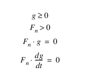
The first three equations reflect:
■The impenetrability constraint
■Separating, normal force constraint
■Requirement that the normal force be nonzero only when contact occurs.
The fourth condition is called the persistency condition and it specifies that the normal force is nonzero only when the rate of separation between the two bodies is zero. The last constraint is particularly important when you are interested in energy conservation or energy dissipation.
You obtain the IMPACT force model by replacing the first three auxiliary contact conditions with the following expression:

where k (stiffness) is a scalar penalty parameter. The penalization becomes exact as k approaches infinity, but otherwise allows small violation of the impenetrability constraint. It is important to note that ill conditioning of the governing equations, and ultimately an integrator failure, will result as the stiffness becomes excessively large. Therefore, you must appropriately select k while preserving the stability of the solution.
You can also approximate the compliance of a body by correlating k to the bodies material and geometric parameters; however, in doing so, you should recall the earlier remark concerning ill conditioning. In an effort to incorporate general material constitutive relationships for the contacting bodies, as well as facilitate time integration, Adams Solver (C++) augments the previous expression with nonlinear displacement-dependent, viscous damping terms. The general form of the IMPACT force function is then given by:
where:
■g represents the penetration of one geometry into another.
■ is the penetration velocity at the contact point.
is the penetration velocity at the contact point.■e is a positive real value denoting the force exponent.
■dmax is a positive real value specifying the boundary penetration to apply the maximum damping coefficient cmax.
Clearly, for cmax = 0 and e = 1, the original penalization is recovered. The POISSON force model is derived from the persistency condition,  . A penalty regularization of the fourth contact constraint yields:
. A penalty regularization of the fourth contact constraint yields:
where p is a scalar penalty parameter. Again, the penalization is exact as  , which carries the risk of ill conditioning. In the context of dynamic contact problems, the POISSON model is more consistent with conservation laws and conserves/dissipates energy appropriately. You can optionally provide a coefficient of restitution e to model inelastic contact. In this case, the POISSON force model computes the normal contact force as follows:
, which carries the risk of ill conditioning. In the context of dynamic contact problems, the POISSON model is more consistent with conservation laws and conserves/dissipates energy appropriately. You can optionally provide a coefficient of restitution e to model inelastic contact. In this case, the POISSON force model computes the normal contact force as follows: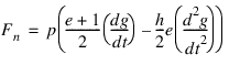
Here, e is coefficient of restitution, g is the penetration depth, and h is the time step.
Contact Friction Force Calculation
Adams Solver (C++) uses a relatively simple velocity-based friction model for contacts. Specifying the frictional behavior is optional. The figure below shows how the coefficient of friction varies with slip velocity.
In this simple model:
■ (-vs) =
 s
s
(-vs) =s ■ (vs) = -
 s
s
(vs) = -s ■ (0) = 0
(0) = 0 ■ (-vd) =
 d
d
(-vd) =d ■ (vd) = -
 d
d
(vd) = -d ■ (v) = -sign(v).
  dfor |v| >vd
(v) = -sign(v). dfor |v| >vd ■ (v) = -step(|v|,vs,
 s, vd,
  d) sign(v) for vs < |v| < vd
(v) = -step(|v|,vs,s, vd, d) sign(v) for vs < |v| < vd■ (v) = step(v,-vs,
 s,vs,-
 s) for -vs < v < vs
(v) = step(v,-vs,s,vs,-s) for -vs < v < vs where:
■V: Slip velocity at contact point
■vs: STICTION_TRANSITION_VELOCITY
■vd: FRICTION_TRANSITION_VELOCITY
■ s: MU_STATIC
s: MU_STATIC■ d: MU_DYNAMIC
d: MU_DYNAMICContact Friction Torque Calculation
If Adams Solver detects an angular velocity about the contact normal axis, it will apply a torque proportional to the friction force. The reason for this is that the contact friction force, by itself, cannot retard relative rotation between bodies; it can only retard relative translation.
Notes: | A slip velocity is necessary to generate contact frictional forces when no stiction is defined for contact friction. In the case of rotational slip, there must be an axis of rotation. The slip velocity increases from zero on the axis (r = 0) to a maximum at the edge of the contact area (r = R). We are using the assumption that the contact area is circular. The slip velocity is used to compute a coefficient of friction (mu). To compute mu in the case of rotation, Adams uses the slip velocity at r = R/2. This can be thought of as the average slip velocity of the entire contact area. This slip velocity is defined as v. The kinematic relationship between the given slip velocity (v) and the corresponding angular slip velocity (w) is: w = v/(R/2) or w = 2v/R The angular slip velocity (w) is used to compute the contact friction torque in the same way translation slip velocity (v) is used to compute the contact friction force. |
The magnitude of the contact friction torque is given by the formula:

Where R is the radius of the contact area (which is assumed to be circular). The coefficient  comes from Marks' Standard Handbook for Mechanical Engineers.
comes from Marks' Standard Handbook for Mechanical Engineers.Caution: | If you need some other formulation of the friction torque, the only alternative is to write your own friction force subroutine (CFFSUB). An example is given at the end of this section. |
Contact Prediction
Contact is fundamentally a discontinuous event. When two geometries come into contact:
■A large normal force or an impulse is generated.
■The velocities of the bodies change sign.
■The accelerations are almost discontinuous, and have a large spike. This spike represents the impulse that was generated due to the contact.
The bodies usually separate because of the contact forces or impulses. Numerical integrators assume that the equations of motion are continuous. A contact event is, therefore, quite hard for an integrator to solve through. Adams Solver (C++) contains a contact predictor that predicts the onset of contact and controls the integrator step size accordingly. The following paragraphs briefly summarize the contact prediction algorithm.
When Adams Solver (C++) detects a new contact, it calculates the penetration and penetration velocity between the two geometries. From these two values, Adams Solver (C++) estimates a more refined contact time. Adams Solver (C++) rejects the current time step and uses the refined step size to accurately sense the onset of contact.
Furthermore, the integrator order is set to one, so that Adams Solver (C++) does not use the time history of the system to predict the future behavior of the system.
This algorithm essentially ensures that:
■The penetration for a new contact is small.
■The integrator is at first order when the contact event occurs.
■The integrator is taking small time steps.
Contacts and Analysis Mode Issues
This section explains how the various analysis modes deal with contact, and provides modeling tips on how to successfully negotiate difficult contact events.
Contacts and Static Equilibrium
Both the static and quasi-static equilibrium analysis modes use Newton-Raphson (NR) iterations to solve the nonlinear algebraic equations of force balance. The Jacobian matrix of first partial derivatives and the residue of the equations of motion are used to set up an iterative scheme that normally converges to the solution.
The Jacobian matrix is a measure of the stiffness matrix of the system. The inverse of the Jacobian is, therefore, the compliance in the system. The NR algorithm ensures that the system solution moves in the direction of most compliance (least stiffness). When a contact is active, the stiffness in the direction of the normal force is high, so the NR algorithm modifies the system states to decrease this force. If a contact is inactive, there is no stiffness in the direction of increasing contact. The NR algorithm will likely compute a large movement in this direction, leading to excessive penetration. During the very next iteration, since the contact force may turn on, a large stiffness is detected in this direction, and the algorithm will change the system to dramatically reduce the amount of penetration. It is not uncommon for the algorithm to overreact to this stiffness and move the system sufficiently to deactivate the contact. The algorithm may never be able to resolve this discontinuity in the system.
Adams Solver (C++) anticipates this situation and uses a contact-force-sensing mechanism to avoid excessive contact. You can further enhance this method, however, by choosing the correct equilibrium parameters.
Here are some modeling tips for aiding equilibrium (static) analysis (for more information on equilibrium analysis, see the EQUILIBRIUM statement):
■If possible, make sure that all contacts are active, and each contact penetration is small. This will ensure that the contact forces are small, and the system is aware of the contacts.
■Set TLIMIT and ALIMIT small enough so gross contact violations are avoided.
■Increase the maximum number of iterations, MAXIT, so that you can get to convergence in spite of the small values for TLIMIT and ALIMIT.
■Avoid neutral equilibrium situations. If you know that your model has neutral equilibrium situations, increase STABILITY (try STABILITY = 0.1). Also increase MAXIT, the maximum number of iterations you will allow to obtain convergence.
■See Best Practices for Working with Contacts for more information.
Contacts and Kinematics
In kinematically determinate systems, the system configuration is completely defined by the system constraints (JOINTs, JPRIMs, COUPLERs, and so on) and MOTIONs. The contact penetration and force at each configuration can only be obtained as outputs of this analysis. CONTACTS will not be able to determine the configuration of the system.
Contacts and Linear Analysis
If contacts are active at the configuration at which linearization is performed, there will be a high stiffness in the direction of the normal force. Therefore, you will see a large frequency corresponding to this stiffness. If contacts are inactive, they will have no effect on the eigenvalues of the system.
Contacts and Dynamics
Default Corrector for Dynamics
The modified corrector (Integrator/Corrector=Modified) is the default for all models that contain CONTACTS.
Handling solution difficulties:
Sometimes, you may encounter repeated corrector failures when a contact occurs. This is usually caused by:
■Too large a value for STIFFNESS (for IMPACT) or PENALTY (for POISSON).
■Too tight of an integration error.
■Too small of a value for FRICTION_TRANSITION_VELOCITY and STICTION_TRANSITION_VELOCITY.
■Too large of a value for MU_STATIC and MU_DYNAMIC.
The following modeling tips will help dynamic analyses. For more information on integrator settings, see the INTEGRATOR statement.
■Reduce STIFFNESS or PENALTY by a factor of 10 and see if Adams Solver (C++) can solve through the contact.
■Increase the integration error tolerance using /ERROR=value. A larger integrator error results in a looser corrector convergence criterion.
■Reduce damping. This decreases the duration of the contact and can help simulations.
■Set the maximum integration order to 2, using INTEGRATOR/KMAX=2. Lower-order integrators are more stable than higher-order integrators.
■Set HMAX to a small value to prevent the integrator from taking large steps.
■Use the SI2 formulation. The corrector for this formulation is more stable than standard GSTIFF, and may solve the problem where the standard GSTIFF failed.
■Always run a model without contact friction first, and refine the functioning model by adding friction later.
■If the addition of frictional forces causes numerical difficulties or simulation slowdowns, gradually increase the values for STICTION_TRANSITION_VELOCITY and FRICTION_TRANSITION_VELOCITY. Also reduce the coefficients of friction, which usually helps the integrator.
Flexible Bodies
Flexible Bodies used in Contacts do not need a corresponding GRAPHICS statement. The geometry for the Flexible Body is extracted from the Modal Neutral File (MNF), which is required.
FE Parts
When an FE Part is selected in Adams View to be used in Contacts, a GRAPHICS object is created.
For 3D FE Parts, the GRAPHICS object is a Parasolid file that represents the surface of the FE Part in its undeformed state. The Parasolid file will be tessellated for contact. The tessellation is updated as the FE Part deforms. 3D FE Part Contact can only be used with the RAPID Geometry Engine. 3D FE Part to 3D FE Part Contact is supported. 3D FE Parts can be used in contact with all 3D geometry except Flex Body. 3D FE Parts cannot be used in Contact with 2D geometry or with 2D FE Parts. When a 3D FE Part contacts a Sphere, the Sphere is treated analytically. No other 3D geometry types are treated analytically.
For 2D FE Parts, the GRAPHICS object is the FE Part centerline. 2D FE Parts can be used in contact with only Curves, Circles and other 2D FE Parts. No other 2D geometry types are supported.
The FE Part must be the IGEOM in all 2D and 3D Contacts, except when FE Part to FE Part Contact is used. Lists of geometry are not supported on the FE Part but they are on JGEOM, when it is not an FE Part.
Caution: | ■An artificially low value of stiffness or penalty will not generate the necessary contact forces. You may see a loss of energy when none is expected. ■If you find that your model response changes as the number of output steps is modified, use INTEGRATOR/HMAX=value to control the integrator step-size and the quality of the solution. ■The HHT integrator is incompatible with restitution (POISSON) contact. If your model uses different length units than the stiffness properties you would like to use, you need to scale the stiffness by: length conversion factor**exponent The reason for this is that the contact force due to penetration is defined as:  Adams View will do this conversion for you if you change the units under Settings. However, you will need to do it if you enter the parameters in different units. Example: k = 3800 N/mm e = 2.0 current model units: force = N, length = m stiffness to enter for contact = 3800*(1000**2) = 3.8e9 Also note that only length is raised to the exponent, so if you have a different force unit, you would only scale it by the force conversion factor. ■Contact cannot be defined between a Flexible Body and a list of 3D geometries ■FLIP cannot be used with flexible bodies ■The edges used in flexible body contact are modeled as 2D polylines. Higher order interpolation is not allowed. Because they are 2D geometry, they may contact any other 2D geometry (rigid or flexible). They cannot be used in contact with 3D geometry. ■The thickness of shell elements is ignored in flexible body contact. |
Tip: | If you notice that energy is dissipated during contact events, note the following: ■Impact method - A three-dimensional contact with zero damping can exhibit some dissipation of energy during the impact. The dissipation is due to the numerics of the integration algorithm. To reduce the dissipation, reduce the time step or tighten (decrease) the error tolerance. ■Restitution method - A three-dimensional contact with coefficient of restitution set to one should conserve energy. If you notice some dissipation, try increasing the PENALTY argument. Recall that the larger the PENALTY argument, the more exact the contact constraint will be enforced. In the case of intermittent contact and a restitution coefficient set to one, a larger penalty parameter more exactly enforces the conservation of momentum during the contact event. The PENALTY argument is analogous to the stiffness in the IMPACT function. The larger the stiffness, the smaller the penetration. Parts with low mass (less than 0.01 kg) may need the PENALTY argument reduced by several orders of magnitude to avoid integrator failures. |
Note: | Solid-to-solid contact is limited to external contact surfaces. So, to take advantage of analytical contact detection for sphere or cylinder geometry and use an internal surface for contact one must specify TYPE = SPHERE_TO_SPHERE or CYLINDER_TO_CYLINDER. |
Material Contact Properties
The table below shows material types and their commonly used values for the dynamic coefficient of friction and restitution.
Material 1: | Material 2: | Mu static: | Mu dynamic: | Restitution coefficient: |
|---|---|---|---|---|
Dry steel | Dry steel | 0.70 | 0.57 | 0.80 |
Greasy steel | Dry steel | 0.23 | 0.16 | 0.90 |
Greasy steel | Greasy steel | 0.23 | 0.16 | 0.90 |
Dry aluminium | Dry steel | 0.70 | 0.50 | 0.85 |
Dry aluminium | Greasy steel | 0.23 | 0.16 | 0.85 |
Dry aluminium | Dry aluminium | 0.70 | 0.50 | 0.85 |
Greasy aluminium | Dry steel | 0.30 | 0.20 | 0.85 |
Greasy aluminium | Greasy steel | 0.23 | 0.16 | 0.85 |
Greasy aluminium | Dry aluminium | 0.30 | 0.20 | 0.85 |
Greasy aluminium | Greasy aluminium | 0.30 | 0.20 | 0.85 |
Acrylic | Dry steel | 0.20 | 0.15 | 0.70 |
Acrylic | Greasy steel | 0.20 | 0.15 | 0.70 |
Acrylic | Dry aluminium | 0.20 | 0.15 | 0.70 |
Acrylic | Greasy aluminium | 0.20 | 0.15 | 0.70 |
Acrylic | Acrylic | 0.20 | 0.15 | 0.70 |
Nylon | Dry aluminium | 0.10 | 0.06 | 0.70 |
Nylon | Greasy aluminium | 0.10 | 0.06 | 0.70 |
Nylon | Acrylic | 0.10 | 0.06 | 0.65 |
Nylon | Nylon | 0.10 | 0.06 | 0.70 |
Dry rubber | Dry steel | 0.80 | 0.76 | 0.95 |
Dry rubber | Greasy steel | 0.80 | 0.76 | 0.95 |
Dry rubber | Dry aluminium | 0.80 | 0.76 | 0.95 |
Dry rubber | Greasy aluminium | 0.80 | 0.76 | 0.95 |
Dry rubber | Acrylic | 0.80 | 0.76 | 0.95 |
Dry rubber | Nylon | 0.80 | 0.76 | 0.95 |
Dry rubber | Dry rubber | 0.80 | 0.76 | 0.95 |
Greasy rubber | Dry steel | 0.63 | 0.56 | 0.95 |
Greasy rubber | Greasy steel | 0.63 | 0.56 | 0.95 |
Greasy rubber | Dry aluminium | 0.63 | 0.56 | 0.95 |
Greasy rubber | Greasy aluminium | 0.63 | 0.56 | 0.95 |
Greasy rubber | Acrylic | 0.63 | 0.56 | 0.95 |
Greasy rubber | Nylon | 0.63 | 0.56 | 0.95 |
Greasy rubber | Dry rubber | 0.63 | 0.56 | 0.95 |
Greasy rubber | Greasy rubber | 0.63 | 0.56 | 0.95 |
Caution: | An artificially low value of stiffness or penalty will not generate the necessary contact forces. You may see a loss of energy when none is expected. If you find that your model response changes as the number of output steps is modified, use INTEGRATOR/HMAX=value to control the integrator step-size and the quality of the solution. |
Best Practices for Working with Contacts
The following list includes tips for working with contacts:
■Step size - Simulations allowed to run at large relative step sizes may cause contacts to have trouble contributing to convergence. Large displacements (especially rotations) during integration steps can cause significant discontinuities. Running with a smaller hmax can help some models by limiting the predictor-induced displacements.
■Equilibrium - Static equilibrium is a very difficult problem to solve with contacts. Use good modeling techniques, such as making sure that the objects expected to be in contact at equilibrium are initially in contact in the input configuration. If this is not feasible, make sure that the objects expected to be in contact are very close so that the contacts can be detected during equilibrium iterations. It will also help to consider the appropriate TLIM and ALIM to help limit the perturbations for finding equilibrium. Use dynamic equilibrium for models that have difficulty finding static equilibrium.
■Thin shells - During one solution step, Adams may take several integrator steps in order to satisfy predictor-corrector requirements. If input geometry is very thin, there is a possibility that one geometry may completely pass through another, resulting in invalid volume of intersection calculations. This can result in missed contacts, passthroughs, or generation of unusually high contact force. Reducing hmax can help prevent this problem.
■Friction - Friction calculations are highly discontinuous and can cause numerical convergence problems, especially at low relative velocities. The friction difficulties compound the already difficult contact evaluations. Whenever possible, run a model without contact friction first, and refine the functioning model by adding friction later. If the addition of frictional forces causes numerical difficulties or simulation slowdowns, gradually increase the values for STICTION_TRANSITION_VELOCITY and FRICTION_TRANSITION_VELOCITY. Also reduce the coefficients of friction, which usually helps the integrator.
■Complex geometry - The time required to retrieve contact intersection information from the geometric modeler is directly related to the complexity of the given geometry. Some methods are deployed to bound geometry to avoid unnecessary calls when possible, but complex geometry can still unduly affect the simulation. Consider the actual contact expected between the geometric pairs. Trim or split the geometry as much as possible to assign contacts to the actual areas of contact interest. Also, when possible, substitute imported or general geometry with geometric primitives, such as cylinders and spheres. These shapes branch into a much faster calculation algorithm.
■Impact versus Restitution - The coefficient of restitution was provided for the case where no impact values were available and restitution values were obtainable from material references or physical testing. In general, the impact method is more numerically smooth and will result in faster simulations. In addition, the impact method provides greater control of the contact behavior, such as inclusion of damping, and force exponent, which can help tune a numerically satisfying result. In general, the coefficient of restitution method should only be used when coefficient of restitution data is available and impact values are not. If a method can be used to derive or determine impact parameters for the given geometry, it should be used. The restitution method is not recommended for Contacts that require friction. The reason is that the Contact friction force is proportional to the normal force and the restitution normal force is nonphysical due to its dependency on acceleration. It is also not recommended to use the restitution method in cases where persistent contact is needed.
■Use Stabilized Index 2 Integrator - The Stabilized Index 2 (SI2) integrator provides better solutions for velocities and derived accelerations without spikes. These acceleration spikes can have adverse effects on contact behavior, so the SI2 integrator is the best choice for most contact models.
■Avoid CONSTANT_BDF (FORTRAN Only) - The constant BDF integrator was created for early design iterations for increased robustness at the cost of accuracy. Models with contacts have been found to perform poorly with constant BDF. Although the model will run more robustly, many observations of contacts missing have been observed.
■2D Approximation for Contact Modeling Whenever Possible - When applicable, represent the contact event using 2D elements. Choose from point-to-curve, curve-to-curve, or use the IMPACT function defined in a SFORCE, VFORCE, or GFORCE element.
■Analytical Contact - Analytical contact should be used whenever possible.
■Contact Parameters (Stiffness, Damping, Force Exponent) - Take into account the mass and inertia of each part in the mechanism and the resulting velocities at which the contact bodies are traveling with respect to each other. Based on this, ensure that the contact parameters are defined with appropriate values.
Examples
The example below demonstrates contact between two generic three-dimensional geometries. star_geneva.xmt_txt is a geometry file that was generated by Parasolid. Adams View or any CAD package using Parasolid as its geometry package can generate this file. It contains two geometries, SOLID4 and SOLID3. Contact is to be defined between these two geometries.
The .adm file portion for this example is as follows:
MARKER/30027, PART = 1005
GRAPHICS/11,
, EXTERNAL,
, FILE = star_geneva.xmt_txt,
, ELEMENT = SOLID4,
, RM = 30027
!
MARKER/30028, PART = 1004
GRAPHICS/12,
, EXTERNAL,
, FILE = star_geneva.xmt_txt,
, ELEMENT = SOLID3,
, RM = 30028
GRAPHICS/11,
, EXTERNAL,
, FILE = star_geneva.xmt_txt,
, ELEMENT = SOLID4,
, RM = 30027
!
MARKER/30028, PART = 1004
GRAPHICS/12,
, EXTERNAL,
, FILE = star_geneva.xmt_txt,
, ELEMENT = SOLID3,
, RM = 30028
An impact-type contact would be defined as:
CONTACT/1,
, IGEOM=11,
, JGEOM=12,
, IMPACT,
, STIFFNESS = 1E6,
, DAMPING = 10,
, DMAX = 0.1,
, EXPONENT = 2.2
, IGEOM=11,
, JGEOM=12,
, IMPACT,
, STIFFNESS = 1E6,
, DAMPING = 10,
, DMAX = 0.1,
, EXPONENT = 2.2
A POISSON-type contact would be defined as:
CONTACT/1,
, IGEOM=11,
, JGEOM=12,
, POISSON,
, PENALTY = 1E5,
, RESTITUTION_COEFFICIENT = 0.6
, IGEOM=11,
, JGEOM=12,
, POISSON,
, PENALTY = 1E5,
, RESTITUTION_COEFFICIENT = 0.6
Below is an example of lists of geometry. Geometries 11 and 12 must belong to one part. Geometries 13, 14, and 15 must all be on one part. Geometries 12, 13, and 15 are flipped.
CONTACT/1,
, IGEOM = 11, 12
, JGEOM = 13, 14, 15
, IFLIP_GEOMETRY = 12
, JFLIP_GEOMETRY = 13, 15
, IMPACT,
, STIFFNESS = 1E6,
, DAMPING = 10,
, DMAX = 0.1,
, EXPONENT = 2.2
, IGEOM = 11, 12
, JGEOM = 13, 14, 15
, IFLIP_GEOMETRY = 12
, JFLIP_GEOMETRY = 13, 15
, IMPACT,
, STIFFNESS = 1E6,
, DAMPING = 10,
, DMAX = 0.1,
, EXPONENT = 2.2
Below is an example of user-written subroutines in contacts. The normal force subroutine (CNFSUB) and the friction force subroutine (CFFSUB) are in the same library (cnforc1).
CONTACT/1
, IGEOM = 7
, JGEOM = 6
, NORMAL_ROUTINE = cnforc1::CNFSUB
, FRICTION_ROUTINE = cnforc1::CFFSUB
, NORMAL_FUNC = USER(1.0E+004, 1.0, 1000, 0.1)/
, FRICTION_FUNC = USER(0.37, 0.30, 10.0, 10)
, IGEOM = 7
, JGEOM = 6
, NORMAL_ROUTINE = cnforc1::CNFSUB
, FRICTION_ROUTINE = cnforc1::CFFSUB
, NORMAL_FUNC = USER(1.0E+004, 1.0, 1000, 0.1)/
, FRICTION_FUNC = USER(0.37, 0.30, 10.0, 10)
The figure below shows a representation of the star_geneva mechanism.
star_geneva Mechanism
The example below demonstrates how to specify contact between two two-dimensional geometries:
MARKER/30027, PART = 1005
GRAPHICS/11, CURVE, RM = 30027, CID = 147
!
MARKER/30028, PART = 1004
GRAPHICS/12, CIRCLE, CM = 30028, RADIUS = 1.36
GRAPHICS/11, CURVE, RM = 30027, CID = 147
!
MARKER/30028, PART = 1004
GRAPHICS/12, CIRCLE, CM = 30028, RADIUS = 1.36
Below is an example of 2D contact for a FLEX_BODY. IEDGE is the ID of a MATRIX statement listing the nodes on the FLEX_BODY which define the edge.
CONTACT/1
, IFLEX = 1
, IEDGE = 2
, JGEOM = 1
, IMPACT
, STIFFNESS = 1.0E+005
, DAMPING = 10
, DMAX = 0.1
, EXPONENT = 2.2
Contact Parameters for Parts with Small Mass
This document gives a method for estimating contact stiffness and damping parameters in Adams for parts with small mass.
The default contact stiffness and damping coefficients in Adams are:
■Stiffness = 1.0E+05 N/mm
■Damping = 10.0 N-s/mm
These coefficients were chosen for parts whose mass is on the order of 1.0 Kg and which are made of steel. Call this part the "default part".
For parts with small mass these coefficients should be reduced to optimize Adams Solver performance and to minimize the chance of simulation failure.
In the following discussion, assume that:
■M = Part mass
■R = Average dimension (size) of part (order of magnitude is sufficient)
■g = gravitational acceleration
■G = G force (1 G = M*g)
Since steel has a density of about 8000 Kg/m^3, the default part would have a radius of about 30 mm (assuming it is spherical).
The expression for the contact spring force is:

where:
■F = Contact force
■K = Contact Stiffness
■x = penetration
■e = exponent (default value in Adams is 2.2)
We would like to calculate the contact force in G's on the default part when its penetration is 0.1% of its radius:

We choose a penetration of 0.1% because most well behaved contact models do not exceed this amount.
To compute the appropriate stiffness for a small part, we specify that it should experience the same G force when it has a penetration of 0.1% of its radius.
Assume the following small part properties:
■M = 4.0e-06 Kg
■R = 1 mm
■e = 2.2
We need to solve the following equation for K:
5*M*g = K*(0.001)^2.2
We get:
When both parts in contact are moving, the reduced mass may give a more accurate estimate of stiffness.
The reduced mass is given by:
The contact damping coefficient for small parts should be calculated using critical damping.
The expression for critical damping is:

For the small part given above, the damping is:

The values for stiffness and damping are order of magnitude estimates. They can be tuned further (via experiment) to refine performance.
Limitations
The contact code in Adams is designed to work with intersection volumes that are "thin", that is, that the penetration squared is less than the area of contact. If this condition is violated, then the contact behavior is unpredictable.
The below rule explains this condition:
If area > 2*d*d then contact force is calculated
If area < 2*d*d then contact force set to zero
where:
■area = contact area
■d = penetration
This condition was added to prevent the contact force from becoming excessively large or from being applied in an unexpected direction.
See other Forces statements available.